---
title: Interpreting Language Model Parameters
authors:
- name: Lucius Bushnaq
affiliation: Goodfire
core_contributor: true
url: https://goodfire.ai
- name: Dan Braun
affiliation: Goodfire
core_contributor: true
equal_contribution: true
url: https://goodfire.ai
- name: Oliver Clive-Griffin
affiliation: Goodfire
equal_contribution: true
core_contributor: true
url: https://goodfire.ai
- name: Bart Bussmann
affiliation: MATS
url: https://goodfire.ai
- name: Nathan Hu
affiliation: MATS
url: https://goodfire.ai
- name: Michael Ivanitskiy
affiliation: MATS
url: https://goodfire.ai
- name: Linda Linsefors
affiliation: Independent
- name: Lee Sharkey
affiliation: Goodfire
core_contributor: true
url: https://goodfire.ai
affiliation: Goodfire, MATS
correspondence: lee@goodfire.com
published: "May 5th 2026"
---
Neural networks use millions to trillions of parameters to learn how to solve tasks that no other machines can solve. What structure do these parameters learn? And how do they compute intelligent behavior?
Mechanistic interpretability aims to uncover how neural networks use their parameters to implement their impressive neural algorithms. Although previous work has uncovered substantial structure in the intermediate representations that networks use, little progress has been made to understand how the parameters and nonlinearities of networks perform computations on those representations.
In this work, we present a method that brings us closer to this understanding by decomposing a language model's parameters into subcomponents that each implement only a small part of the model's learned algorithm, while simultaneously requiring only a small fraction of those subcomponents to account for the network's behavior on any input.
The method, adVersarial Parameter Decomposition (VPD), optimizes for decompositions of neural network parameters into simple subcomponents that preserve the network's input-output behavior even when many subcomponents are ablated, including under ablations that are adversarially selected to destroy behavior. This encourages learning subcomponents that provide short, mechanistically faithful descriptions of the network's behavior that should aggregate appropriately into more global descriptions of the network's learned algorithm.
We study how sequences of interactions between these parameter subcomponents produce the network's output on particular inputs, enabling a new kind of 'circuit' analysis. While more work remains to be done to deepen our understanding of how neural networks use their parameters to compute their behavior, our work suggests an approach to identify a small set of simple, mechanistically faithful subcomponents on which further mechanistic analysis can be based.
## Introduction
Mechanistic interpretability aims to reverse engineer neural networks, such as language models, so that we can understand the neural algorithms they have learned. Reverse engineering requires decomposing a system into simpler parts that we can study in relative isolation. Unfortunately, it is not obvious how best to decompose neural networks into such parts mueller2024questrightmediatorhistory, sharkey2025openproblemsmechanisticinterpretability.
The most straightforward candidates for these parts, such as neurons, attention heads, or whole layers, don't always map to individual, interpretable computations hinton1981parallel, wei2015understandingintraclassknowledgeinside, nguyen2016multifacetedfeaturevisualizationuncovering, olah2017feature, janiak2023polysemantic, jermyn2023attention, yun2021sparse, lindsey2024crosscoders.
Alternative approaches to decomposition, such as transcoders dunefsky2024transcodersinterpretablellmfeature, ameisen2025circuit or mixtures of linear transforms oldfield2025towards, lindsey2025molts, typically involve fitting a set of simple functions to the transitions between activations at different layers in the network, and linearly combining the outputs of these simple functions.
The idea here is to approximate the complex, nonlinear function implemented by the network's layers using a simpler, easier-to-understand function. These methods, sometimes called *activation-based decomposition* methods, have led to significant advances in our understanding of the intermediate representations inside neural networks when computing their outputs dunefsky2024transcodersinterpretablellmfeature, ameisen2025circuit.
Unfortunately, because the simpler functions that these methods use are of a different functional form to the original network, it is hard to relate their accounts of network function to the actual objects that are doing the computations, namely the network's parameters and nonlinearities.
This is not just a theoretical issue. It prevents us from achieving practical engineering goals. For example, it makes it challenging to know how to make precise, predictable modifications to a model's neural algorithm by making edits to its parameters. It also makes it hard to predict how the model's neural algorithm will perform on a different distribution to the one it was studied on.
The mismatch of functional form between models and their activation-based decompositions is an important issue, but it is not the only one: Activation-based methods have not yet yielded decompositions that exhibit a fully satisfactory level of mechanistic faithfulness ameisen2025circuit, and suffer from a number of other issues (See sharkey2025openproblemsmechanisticinterpretability for review).
These issues motivate alternative approaches to mechanistic decomposition, including parameter decomposition methods braun2025interpretabilityparameterspaceminimizing, bushnaq2025spd, chrisman2025identifyingsparselyactivecircuits, which give accounts of network function in terms of the parameters that the network uses on each datapoint. *Ablation-based parameter decomposition methods* braun2025interpretabilityparameterspaceminimizing, bushnaq2025spd aim to identify a set of parameter components where as few components as possible are necessary to perform the same computations as the original network on any datapoint, and "unnecessary" components can be ablated on a given datapoint in any combination without adversely affecting output reconstruction error. Simultaneously, the parameter components are selected to implement as simple computations as possible and to sum collectively to the target network's parameters. If parameter components exhibit all these properties, then they are strong candidates for the network's 'ground truth' mechanismsThough one would first need to accept philosophically that such mechanisms can be said to exist in non-toy networks!.
Parameter decomposition methods can identify known ground truth mechanisms in toy models that: Are not necessarily aligned to architectural components such as neurons, individual attention heads, or layers; operate on representations in superposition; or are multidimensional. And, due to the requirement that unnecessary components can be ablated in any combination rather than just all simultaneously, parameter decomposition methods should not exhibit feature splitting. Notably, parameter decomposition methods can readily be applied to any architecture, unlike activation-based methods, where it has been challenging to use the same decomposition methods to decompose both attention layers and MLPs kamath2025tracing, ameisen2025circuit, wynroe2024decomposing, ge2024localglobal. In demonstration of this ability, previous work has used ablation-based parameter decomposition to identify induction heads in a transformer trained on a toy model of induction christensen2025decomposition.
Ablation-based parameter decomposition methods thus promise solutions to many of the issues of activation-based decomposition methods. However, prior parameter decomposition proposals have several important shortcomings, some of which we address in this work with a new method that we introduce, called *ad**V**ersarial **P**arameter **D**ecomposition* (**VPD**)Regrettably, the acronym APD was taken by our previous work, Attribution-based Parameter Decomposition!braun2025interpretabilityparameterspaceminimizing. Our main contributions are:
- **We scale parameter decomposition to full language models**: While the most recent parameter decomposition method, Stochastic Parameter Decomposition (SPD)bushnaq2025spd is more scalable than its predecessor, Attribution-based Parameter Decomposition braun2025interpretabilityparameterspaceminimizing, it has not yet been applied to full language models. We use VPD to decompose a small language model ($67$M parameters, four layers) trained on the Pile gao2020pile. We find parameter subcomponents that are highly interpretable (sec:param-comps-interpretable), both in terms of the dataset examples that they activate on and how they interact with other subcomponents to produce specific behaviors (sec:circuits).
- **We introduce a stronger notion of ablatability to achieve more mechanistic faithfulness**: While some work has applied SPD to a single layer of GPT2-small christensen2025decomposition, no application of SPD so far has measured key metrics that would be necessary to ensure mechanistic faithfulness, such as having good output reconstruction loss even under adversarially chosen ablations (rather than under only stochastically chosen ablations). We resolve this issue with VPD, which builds heavily on the SPD method but has several important modifications, which together make it more mechanistically faithful and scalable to larger models than those decomposed in previous work. The primary difference between VPD and SPD is in the ablations. On each datapoint, both SPD and VPD sample from the space of possible partial ablations of parameter subcomponents in order to check whether those parameter subcomponents can be partially ablated in any combination, thus identifying whether they are "necessary" for that datapoint. However, where SPD samples from the space of partial ablations using *stochastic* samples from the space, VPD uses *adversarially chosen samples* (sec:opt-mech-faithfulness) Both approaches are nonetheless designed to approximate what would happen if we could check *all* potential partial ablations.. The core details of the method are discussed in sec:method.
- **We compare VPD to other decomposition methods**: We compare the parameter subcomponents that we find to the objects found by other decomposition methods, such as per-layer and cross-layer transcoder (CLT) latents. We find that VPD achieves a better tradeoff between sparsity and reconstruction under standard training objectives and is more robust to mismatches between training and evaluation protocols compared to end-to-end trained methods (sec:decomp-model-behav-sim, app:vpd-sparsity-acc-tradeoff). VPD also has comparable interpretability (sec:param-comps-interpretable) and exhibits less feature splitting (sec:splitting) than activation-based comparisons.
- **We decompose attention layers into computations that are distributed across multiple heads**: Our approach decomposes parameters in attention layers into functionally specialized subcomponents that span multiple heads. These subcomponents interact to perform interpretable computations. Perhaps for the first time, our approach yields a satisfying decomposition of computations in attention layers even though those computations may involve multiple heads (sec:attn-analysis).
- **We develop attribution graphs to study information flow between parameter subcomponents**: We demonstrate that the parameter subcomponents found by VPD can be used to construct interpretable attribution graphs that let us study the circuits that underlie some language model behaviors (sec:circuits).
- **We use parameter subcomponents to manually edit a model**: Finally, we provide a proof of concept showing that we can use our understanding of the network’s parameters to manually edit a model in a predictable, interpretable way. In particular, we rewrite the part of its neural algorithm involved in emoticon predictions (sec:model-editing).
Additionally, we also introduce an approach for clustering parameter subcomponents into full parameter components. Previous methods left this clustering step implicit bushnaq2025spd (app:clustering). We introduce an explicit clustering method, but found that subcomponents were usually interpretable even without clustering, and therefore used clustering only rarely in our analyses.
We release a library for reproducing our experiments and running VPD at https://github.com/goodfire-ai/param-decomp.
## The core method: adVersarial Parameter Decomposition {toc: Method: adVersarial Parameter Decomposition}
In this section, we introduce ablation-based parameter decomposition methods from scratch and highlight key differences between VPD and prior methods in this class. Although our method, VPD, builds heavily on SPD bushnaq2025spd, the following explanation of VPD does not assume familiarity with SPD or its predecessor braun2025interpretabilityparameterspaceminimizing.
Our goal is to decompose a neural network into the *mechanisms* that it uses to compute its behavior. Its mechanisms are what it uses to take input activations, compute its hidden activations, and finally compute its output. We don't approach this goal with strong presuppositions of what a "mechanism" is. But we take for granted that a typical network doesn't use all of its mechanisms on every input (or, at least, it doesn't use all of its mechanisms by the same amount). If that were not the case, then networks could not be said to be *modular*, having distinct parts that do different things on different inputs. Without modularity, networks simply couldn't be decomposed into separable functional units.
One candidate for the network's mechanisms is the network's parameters. Like mechanisms, networks appear not to use all of their parameters simultaneously on every datapoint veit2016residual, zhang2022moefication, dong2023attention. This happens, for instance, when a network's parameters "read from" activation subspaces that are orthogonal to the activations on that datapoint, thus projecting the activations to zero, thereafter having no downstream causal effect. Alternatively, if the activations fail to "activate" a given ReLU neuron, the activation of that neuron is zero, thereafter having no downstream causal effect. However, the network's parameters are in fact a single vector in the network's parameter space, and do not have an obvious decomposition into parts. How should they be decomposed into parts that comprise the network's mechanisms?
On a high level, parameter decomposition methods use the idea that it should be possible, for a given datapoint, to identify the "subset" of the network's parameters that are necessary and sufficient for computing its output on that datapoint. That "subset" of parameters should contain all the mechanisms used by the network on that datapoint. If particular "subsets" of the network's parameters are repeatedly used together by different datapoints, then they may be part of the same mechanism. Parameter decomposition methods therefore aim to find particular "subsets" of the network's parameters that tend to be used together, where as few of them as possible are necessary and sufficient for computing the network's output on any inputWe use the word "subset" loosely here. In practice, parameters are not divided into discrete sets. The network's parameters are a vector in parameter space, and we want some way to divide up that vector into 'parts' in a way that they still 'make up' the original parameters..An analogy that is sometimes helpful for understanding VPD is that it is similar to Singular Value Decomposition on a weight matrix, except where we decompose the matrix into more subcomponents than the rank of the matrix, and where the subcomponents we identify are the parts of the matrix that have similar downstream causal effects, thereby taking downstream nonlinearities into account.
More concretely: If particular parameters are unused by the network on a particular datapoint, then we should be able to ablate them (including partially) on that datapoint without adversely affecting the network's output. Ablation-based parameter decomposition methods thus aim to decompose network parameters into a set of vectors in parameter space called *parameter components*. Parameter components are trained to exhibit a number of specific properties such that, if they exhibit those properties, they would be good candidates for the network's "mechanisms". They are trained to be:
- **Parameter-faithful**: They sum to the network's total parameter vector;
- **Minimal**: As few components as possible are causally important for computing the network's output on any particular input;
- **Mechanistically faithful**: Every subset of components that includes the causally important components is sufficient to compute the network's output on any particular input;
- **Simple**: Each component should involve as little computational machinery as possible.
In the following sections, we define parameter components concretely and explain how they are optimized to exhibit each of these four properties.
### Parameter components consist of subcomponents {toc: Subcomponents}
Suppose we have a neural network $f(x;\theta)$ with parameters $\theta$. We would like to decompose this parameter vector into a sum of *parameter components* with the above properties.
It would be computationally expensive to decompose models into whole parameter vectors, since each such vector would have a memory cost equivalent to the whole target model. Therefore, as in bushnaq2025spd, we use a less expensive way to parameterize parameter components: Although its parameters $\theta$ can be expressed as a single large vector, they are more commonly conceptualized as a set of matrices $\theta = \{W_1, \dots, W_L\}$. We further decompose individual matrices into sums of rank-one matrices called *subcomponents*, each parameterized as an outer product of two vectors:
$$W_l \approx \sum_{c} \vec{U}^l_c (\vec{V}_c^l)^\top = U^l (V^l)^\top , $$
where there may be more subcomponents than rows and columns in the matrix. Permitting more subcomponents than rows and columns in the matrix allows VPD to identify mechanisms that operate on representations in superpositionVaintrob_Mendel_Kaarel_2024, Bushnaq_Mendel_2024, elhage2022toy.
Parameter decomposition methods decompose target model parameters into vectors in parameter space (parameter components) that are optimized to approximate the model's mechanisms.
Although a single subcomponent *explicitly* parameterizes only a single weight matrix, it *implicitly* parametrizes a full parameter vector if we assume it takes values of $0$ in all other weight matrices. It is therefore possible to combine these subcomponents into full parameter components by adding them together in the right way. We identify these components using a subcomponent clustering method. Previous work left this clustering step implicit, but in this paper we introduce an explicit method (app:clustering).
### Enforcing parameter faithfulness with $\Delta$-components {toc: Enforcing parameter faithfulness}
To ensure the components collectively sum to the parameter vector of the target model, we define additional $\Delta$-components, $\Delta^l$, that parametrize the difference between our subcomponents and the original model's matrices:
```equation
label: eq:delta_l2
tex:
\htmlClass{hc-dl-delta}{\Delta^l}
:=
\htmlClass{hc-dl-W}{W^{l}}
-
\htmlClass{hc-dl-summed}{
\sum_{c}
\htmlClass{hc-dl-uv}{\vec{U}^l_c (\vec{V}_c^l)^\top}
}
tips:
- hc-dl-delta: The Δ-component for target model parameter matrix l
- hc-dl-W: Target model parameter matrix l
- hc-dl-summed: The summed parameter subcomponents
- hc-dl-uv: Rank-1 parameter subcomponent c for matrix l
```
We also encourage the $\Delta^l$-components to be small with an auxiliary MSE loss ($\mathcal{L}_{\text{Delta-L2}}$) (sec:vpd_delta_l2).
### Optimizing for minimality
We want as few subcomponents as possible to be causally important for computing the network's output on any particular input. We therefore need some way to estimate which parameter subcomponents are "necessary" for computing the network's output on a given datapoint. We also require a notion of how well the "necessary" subcomponents have reconstructed the network's output.
Ablation-based parameter decomposition methods contend that a parameter subcomponent is "necessary" if it cannot be ablated without affecting the model's output on that datapoint. As in bushnaq2025spd, we train a *causal importance function* to predict how ablatable each subcomponent is on each batch and sequence position. We also implement the causal importance function using a neural network, though we use a different architecture (sec:vpd_ci_function).
We call the output of this function the *causal importance values*, $g^l_{b,t,c}\in[0,1]$ (for each subcomponent $c$ of weight matrix $l$ at a given batch index $b$ and sequence position $t$):
- If $g^l_{b,t,c} = 0$, then we should be able to fully or partially ablate that subcomponent on the forward pass at position $b,t$ without affecting the final model output.
- If $g^l_{b,t,c} = 1$, then it should not be possible to ablate that subcomponent without affecting the model's output on that datapointThe Delta-components $\Delta^l$ should always be ablatable, so they are assigned a causal importance of $0$ by definition..
We want as few subcomponents as possible to be required to compute the output, so we train the causal importance values $g^l_{b,t,c}$ to take minimal values with an *importance minimality loss*:
$$
\begin{aligned}
\mathcal{L}_{\text{importance-minimality}}
=
\frac{1}{BT}
\sum^{B}_{b=1}
\sum^{T}_{t=1}
\sum^{L}_{l=1}
\sum^C_{c=1}
\vert g^l_{b,t,c} \vert^p,
\end{aligned}
$$
where $p>0$.The $\Delta^l$-components are defined always to have causal importance values of zero, since they should never be "necessary" to compute the model output.
### Optimizing for mechanistic faithfulness
Components and their causal importances should be mechanistically faithful to the original model. One way of operationalizing this is to insist that, on any given data point, it should ideally be possible to ablate all causally unimportant components from the model weights, using any combination of ablations, without changing the model output. Another, more succinct, way of saying this is that *every* subset of components that includes the causally important components should be sufficient to compute the network's output on any particular input.
This is a much stricter requirement than merely demanding that the output should be invariant to the joint ablation of all causally unimportant components together. To see why it is stricter, suppose that two components $\theta_A$ and $\theta_B$ can be *jointly* ablated, but not *individually* ablated, on a data point without affecting the output One way this could happen if $\theta_A$ and $\theta_B$ cancel each other out by influencing the final model output vector in opposite directions.. Then we would consider both $\theta_A$ and $\theta_B$ to be causally important on that datapoint, whereas the less strict criterion might consider them both causally unimportant because they happen to be jointly ablatable. In other words, the stricter criterion demands an unchanged model output over a whole set of points in parameter space, whereas the less strict one demands it only for a single point. For an illustration of why this stricter condition is necessary, see sec:vpd_recon_motivation.
VPD works on the level of rank-1 subcomponents instead of full components, but the same principle applies. Demanding that every combination of causally unimportant subcomponents is ablatable is actually stricter than demanding that every combination of causally important components is ablatable. See sec:limitations for some discussion of this. To check whether subcomponents are ablatable, we define ablation masks $m^l_{b,t,c}\in[g^l_{b,t,c},1]$ for each subcomponent at each batch index $b$ and sequence position $t$. So, if a subcomponent has causal importance $g^l_{b,t,c}=1$, the only permitted value for the mask $m^l_{b,t,c}$ is also $1$, whereas if the causal importance is $0$, its mask can take any value between $0$ and $1$. These masks define new weight matrices $W^{\prime l}_{b,t}$ which we should be able to insert in place of the original model matrices $W^l$ without substantially changing the model's final output.
We operationalize this by demanding that the KL-divergence $D$ between the model output on the original forward pass and on forward passes using the masked weights should be small:
```equation
label: eq:random_recon
tex:
\begin{aligned}
\mathcal{L}_{\text{masked-recon}}
&=
\frac{1}{B}
\sum^{B}_{b=1}
\htmlClass{hc-stoch_rec-divergence}{
D
\Big(
\htmlClass{hc-stoch_rec-target_output}{
f(
\vec{x}_b
\vert
\htmlClass{hc-stoch_rec-target_weight}{
W^1,\dots,W^L
}
)
}
,
\htmlClass{hc-stoch_rec-stoch_output}{
f(
\vec{x}_b
\vert
\htmlClass{hc-stoch_rec-w_stoch}{
{W'}^1_b(
m^1
),\dots,{W'}^L_b(
m^L
)
}
)
}
\Big)
} \\
\end{aligned}
tips:
- hc-stoch_rec-divergence: The KL-divergence between the target model and the masked model.
- hc-stoch_rec-stoch_output: The decomposed model's output on datapoint $\vec{x}_b$
- hc-stoch_rec-w_stoch: The weight matrix created by masking parameter subcomponents and Delta components
- hc-stoch_rec-target_output: The target model's output on input datapoint $\vec{x}_b$
- hc-stoch_rec-target_weight: The target model's weights
```
Ideally, we would calculate this masked reconstruction loss for every permitted combination of ablation masks $m$ for all subcomponentsAnd Delta components. in all the model's weight matrices, but this would require performing an intractably large number of forward passes. So we instead use ablation masks $m$ drawn using two types of sampling:
1. **Stochastic sampling**, with ablation masks $m^{\text{stoch}}$ drawn from uniform distributions. This yields the *stochastic reconstruction loss*, $\mathcal{L}_{\text{stochastic-recon}}$.
2. **Adversarial sampling**, using ablation masks $m^{\text{adv}}$ optimized via gradient ascent to maximise the reconstruction loss. This yields the *adversarial reconstruction loss*, $\mathcal{L}_{\text{adversarial-recon}}$.
For details on the stochastic and adversarial sampling, see sec:recon.
### Optimizing for simplicity
Each component ought to contain as little computational machinery as possible. Otherwise, we could say that the target model is one big parameter component, and proclaim our decomposition complete without doing any actual decomposition!
We both constrain and train our subcomponents to be simple. Our subcomponents are rank-one, which constrains them to be simpler objects than full matrices. Unfortunately, this is not enough of a simplicity constraint, because some rank-one solutions can be "simpler" than others: In some situations, it is possible to add multiple subcomponents parametrizing independent mechanisms used on disjoint subsets of the data together and have the resulting sum also be rank-one. We observed indications that some VPD decompositions suffered from this failure mode. Sometimes, subcomponents seemed to be involved in multiple (usually two) unrelated computations, which depended on whether the incoming activations had strong positive or negative inner products with the subcomponent's right singular vector.A theoretically clean motivating example of this phenomenon is the toy model of ping pong superposition gibson2025. In the ping pong superposition construction, $64$ superposed rank $1$ circuits can be implemented in layers of width $21$. Only one circuit is ever active at a time, and groups of eight circuits each share the exact same origin or target neurons. Subcomponents for circuits in the same group can then be summed, and the result will again be exactly representable as a rank $1$ matrix, which is causally important for computing the output exactly when any of the circuits in the group are causally important for computing the output. Hence if we apply VPD to this toy model, the importance minimality loss alone will provide no incentive to further separate the eight rank $1$ matrices for the eight circuit groups into $64$ rank $1$ matrices for the $64$ individual circuits, leaving us with components that activate polysemantically and contain more computational machinery than they need to.
We therefore encourage breaking up subcomponents into multiple that are causally important on as few data points as possible by introducing an additional, slightly superlinear, penalty on subcomponent activation frequency:
```equation
label: eq:freq_minimality
tex:
\begin{aligned}
\mathcal{L}_{\text{frequency-minimality}}
=
\frac{1}{B T}
\sum^{B}_{b=1}\sum^{T}_{t=1}\sum^L_{l=1}\sum^C_{c=1}
\htmlClass{hc-g-left}{\vert g^l_{b,t,c} \vert^p}
\htmlClass{hc-g-right}{
\log_2(
1 +
\sum^{B}_{b'=1}\sum^{T}_{t'=1}
\vert
g^l_{b',t',c}
\vert^p
)},
\end{aligned}
tips:
- hc-g-left: This term is just the causal importance set to the p^th power, similar to the importance minimality loss
- hc-g-right: This term sums over the batch and is therefore higher for higher frequency subcomponents
```
There are probably multiple ways to optimize for the computational simplicity of parameter subcomponents, and we are not confident this choice is optimal (nor our choices for the other losses). Nonetheless, we found it to work well enough in practice. See sec:vpd_frequency_penalty for a more detailed motivation of this loss.
### Summary of loss terms
In total, our loss function has five terms:
$$
\begin{aligned}
\mathcal{L}_{\text{VPD}} ={}
& \beta_1 \mathcal{L}_{\text{adversarial-recon}} \\
+ & \beta_2 \mathcal{L}_{\text{stochastic-recon}} \\
+ & \beta_3 \mathcal{L}_{\text{importance-minimality}} \\
+ & \beta_4 \mathcal{L}_{\text{frequency-minimality}} \\
+ & \beta_5 \mathcal{L}_{\text{Delta-L2}}
\end{aligned}
$$
They each optimize the parameter subcomponents to exhibit particular properties:
- The $\mathcal{L}_{\text{adversarial-recon}}$ and $\mathcal{L}_{\text{stochastic-recon}}$ losses optimize for **mechanistic faithfulness** (eq:random_recon).
- The $\mathcal{L}_{\text{importance-minimality}}$ loss optimizes for **minimality** (eq:minimal).
- The $\mathcal{L}_{\text{frequency-minimality}}$ loss optimizes subcomponents for **simplicity**. They are also constrained to be rank-1 matrices, which imposes one aspect of simplicity (eq:freq_minimality).
- The $\mathcal{L}_{\text{Delta-L2}}$ auxiliary loss optimizes for **parameter-faithfulness**, even without the $\Delta$-components, which ensure it (eq:delta_l2).
The key difference between VPD and our previous work bushnaq2025spd is the $\mathcal{L}_{\text{adversarial-recon}}$ and $\mathcal{L}_{\text{frequency-minimality}}$ losses. There are several other, smaller differences that do not fundamentally change the method but that we found helpful for decomposing language models. For more details, see sec:vpd_methods.
We evaluate the quality of our decomposition on a number of key metrics. For assessing the quality of a decomposition, the most important are $\mathcal{L}_{\text{adversarial-recon}}$ and $L_0$ per datapoint. For readers looking for practical advice on how to tune hyperparameters and key optimization metrics, we provide a detailed *Training recipe for VPD* in app:recipe.
## Analyzing language model parameter subcomponents {toc: Analyzing subcomponents}
### Target language model
We trained a four-layer 67M parameter decoder-only transformer model on an uncopyrighted subset of The Pile gao2020pile. A summary of the model architecture and training results can be found in tab:model-hyperparams and full training details of our target model can be found in app:training-details.
Our target model is a standard decoder-only transformer language model.
| Attributes of our target model | |
|---|---|
| Layers | 4 |
| Residual stream dimension | 768 |
| MLP intermediate dimension | 3072 |
| Attention heads | 6 |
| Attention head dimension | 128 |
| Context length | 512 |
| Vocabulary size | 50,277 |
| Positional encoding | RoPE su2024roformer |
| Normalization | RMSNorm zhang2019rootmeansquarelayer |
| Activation function | GELU hendrycks2016gelu |
| Attention type | Standard Multi-Head Attention vaswani2017attention |
| Tied embeddings | Yes |
| Non-embedding parameters | ~28M |
| Total parameters (incl. embedding) | ~67M |
| Training dataset | The Pile gao2020pile (subset) |
We decomposed the 24 weight matrices in this model into a total of of 38,912 rank $1$ subcomponents. We omitted the embedding and unembedding matrices. The decomposition used much fewer than its full capacity, having only ~10,000 alive components (with a mean causal importance greater than $10^{-6}$).
On average, each datapoint uses 205 subcomponents per sequence position, representing 2.1% of all alive subcomponents. tab:num-components-per-layer shows per-layer summary statistics for the decomposition.
| Layer | $C$ | Alive | Mean L0 | L0/Alive |
|---------|---------|--------|--------------|--------------|
| Layer 0 | $9728$ | $3709$ | $44.6$ | $0.012$ |
| Layer 1 | $9728$ | $848$ | $18.9$ | $0.022$ |
| Layer 2 | $9728$ | $1943$ | $49.5$ | $0.025$ |
| Layer 3 | $9728$ | $3472$ | $92.0$ | $0.026$ |
| Total | $38912$ | $9972$ | $205.0$ | $0.021$ |
Table: Per-layer decomposition summary statistics: Subcomponent dictionary sizes $C$; alive subcomponents (subcomponents with mean causal importances above $10^{-6}$ at the end of training); average $L_0$ scores of subcomponents with causal importance $>0$ per batch and sequence position; and fraction of all subcomponents with causal importance $>0$ per batch and sequence position.
### The decomposition model behaves similarly to the target model {toc: Decomposition model behavior}
If a decomposition method has correctly identified the mechanisms underlying a model's computation, then activating only the mechanisms that the method identifies as causally important on a given input should approximately reproduce the model's behavior on that input. Conversely, if a replacement model fails to reproduce the model's behavior, then the decomposition has either missed important mechanisms or identified spurious ones. Reconstruction quality is therefore a necessary (though not sufficient) condition for a decomposition to be mechanistically faithful.
Our parameter subcomponents capture different amounts of the target model's performance depending on how masks are calculated (tab:vpd-ce-compute-compar). One quantitative measure of performance is cross-entropy (CE) loss on the validation set: The decomposed model achieves between 2.72 and 3.02, depending on the type of sampling, compared with 2.71 for the target model.
A metric that is sometimes helpful for comparison is *Pretraining Compute Recovered*gao2024scalingevaluatingsparseautoencoders, which is the percentage of the target model's total pretraining compute at which the target model's training curve reaches the same validation CE loss as the reconstruction model (i.e. a value of X% means the reconstruction performs no better than the target model did when only X% of pretraining was complete).
When we exclude the $\Delta$-component (which is trained to be as causally unimportant as possible), the remaining *unmasked* parameter subcomponents recover about $82\%$ of the pretraining compute. When using stochastic ablations, this drops to around $27\%.$
| Masking mode (excluding $\Delta$-components) | Validation CE Loss | Pretraining Compute Recovered (%) |
|:---------------------------------------------|-------------------:|:--------------------------------|
| **Target Model** | **2.71** | **100%** |
| Unmasked (All masks$=$1) | 2.72 | 82.4% |
| Stochastic Masks | 2.84 | 26.9% |
| Rounded Masks (Mask$=$1 if CI$>$0) | 2.94 | 11.8% |
| Rounded Masks (Mask$=$1 if CI$>$0.1) | 2.95 | 11.3% |
| Causal Importance values (CIs) used as Masks | 2.99 | 9.4% |
| Rounded Masks (Mask$=$1 if CI$>$0.5) | 3.02 | 8.0% |
Pretraining compute recovered is rarely reported, so comparisons to other methods are difficult. Nonetheless, VPD compares favorably to the only other method in the literature that we are aware of that reports this metric: Top-$k$ SAEs gao2024scalingevaluatingsparseautoencoders reports a pretraining compute recovered of $10\%$ when replacing a single layer of GPT-4 with an SAE with 16 million latents. By comparison, even though our approach decomposes the whole model rather than just a single layer, it recovers between $8\%$ and $27\%$, depending on the ablation method usedNote, however, that comparing this metric across models assumes similar levels of compute optimality for both decomposed models, which may not be the case. .
The table below shows KL-divergence to the target model under adversarial masking with different numbers of adversarial optimization steps, calculated across a batch of $128$ of sequence length $512$ drawn from the evaluation set The adversarial masks were calculated with Projected Gradient Descent (PGD)madry2018towards optimization, sharing the same source for each subcomponent across the batch. For more details on the PGD loss evaluation metric see sec:vpd_methods-adv..
| Adversarial optimization steps $n^{\text{adv}}$ | KL divergence to target model |
|:-------------------------------|----------:|:-----------------------------|
| 20 | 0.8280 |
| 40 | 1.3539 |
| 80 | 3.8381 |
| 160 | 25.2560 |
| 320 | 40.2200 |
While the decomposition is somewhat robust to approximately $20$ steps of adversarial optimization, it is clearly not at all robust to $160$ steps or more. To provide some sense of scale, zero-ablating all of the target model's weight matrices gives a KL-divergence of ca. $67.2449$.
However, we note that *complete* adversarial robustness would not necessarily be desirable. See sec:vpd_recon_motivation for some discussion of how much adversarial robustness a decomposition ought to exhibit to be considered mechanistically faithful.
Qualitatively, the generations produced by different sampling methods align with the above quantitative measures. The generations seem qualitatively to produce similar behavior to the target model in most cases (fig:generations-showcase).
```generations
data: data/generation_comparisons.json
caption: Side-by-side generation comparisons across masking strategies.
```
Surprisingly, even when masks are adversarially sampled with 20 steps of adversarial optimization, the generations are not *entirely* nonsensical. This is feasible because we only get to adversarially sample causally unimportant parameter subcomponents.
### VPD has a better tradeoff between reconstruction versus sparsity compared with transcoders {toc: Comparison with transcoders}
Any decomposition of a neural network faces a fundamental tradeoff between the number of `objects' they use to reconstruct the network's behavior and the quality of that reconstruction. If a decomposition can use fewer objects to capture the same amount of network performance, then that explanation is preferred according to Occam's razor, assuming the objects use a similar amount of computational machinery.
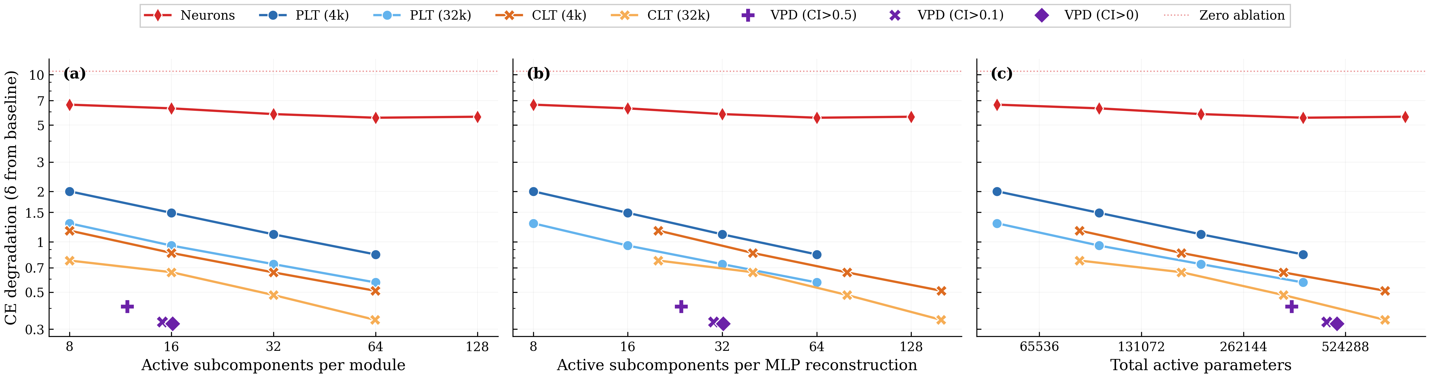
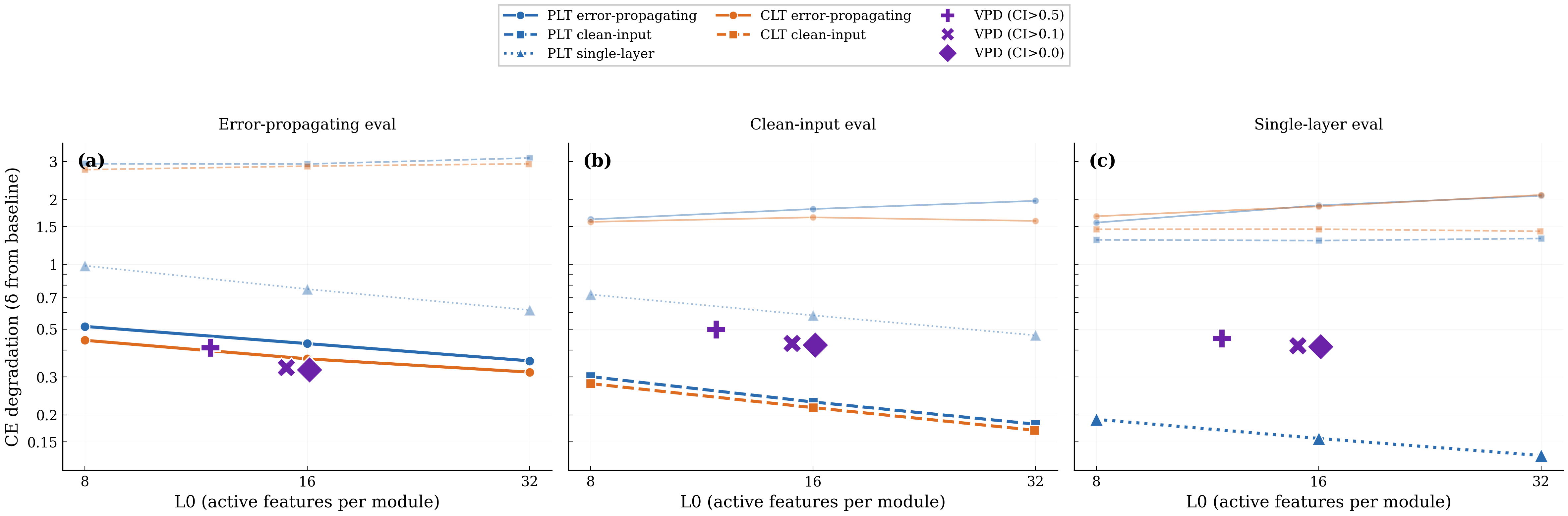
We study the reconstruction versus sparsity tradeoffs of different decompositions and compare the VPD model with two families of activation-based decomposition methods: Per-layer transcoders (PLTs) dunefsky2024transcodersinterpretablellmfeature and cross-layer transcoders (CLTs) lindsey2024crosscoders, both using BatchTopK bussmann2024batchtopk. We simultaneously replace all 4 MLP layers of the target model with their sparse reconstructions and measure the resulting increase in cross-entropy loss relative to the unmodified target model.
There isn't a straightforward apples-to-apples comparison between transcoder latents and VPD subcomponents, so we present a number of different comparisons (with more extensive experimental details in app:vpd-sparsity-acc-tradeoff) Comparing sparsity across methods requires care, because each method has structurally different notion of what constitutes a single active element. A CLT feature writes to the residual stream at every layer simultaneously, while a PLT latent affects only one layer. VPD subcomponents are scoped to individual weight matrices, and each MLP layer has two such matrices ($W_{\text{in}}$ and $W_{\text{out}}$).. To ensure our conclusions are not artifacts of how we count subcomponents or latents, we show results under three possible definitions of sparsity:
1. **Average active subcomponents per module**: Active encoder latents for PLTs/CLTs; active subcomponents per weight matrix for VPD;
1. **Active subcomponents per MLP Down reconstruction**: Adjusting for the fact that a CLT latent affects multiple layers and that VPD uses two modules per MLP;
1. **Total active parameters**: VPD's rank-one subcomponents have more parameters than a PLT latent and a single CLT latent has multiple decoder vectors.
We compare VPD with PLTs and CLTs trained with their standard training losses, noting these are different objectives (VPD trains on output reconstruction while PLTs and CLTs are trained to reconstruct activations at each layer).
CE degradation when simultaneously replacing all 4 MLP layers with sparse reconstructions from each method. **(a)** Active subcomponents per module (raw L0). **(b)** Active subcomponents per MLP reconstruction, adjusting for CLT's cross-layer writes and VPD's paired modules. **(c)** Total active parameters. VPD (purple markers) Pareto-dominates the activation-based methods under all three sparsity measures. The dashed line indicates zero-ablation (all MLP outputs set to zero). Lower is better.
We observe that VPD performs favorably compared with activation-based decomposition, achieving less CE degradation for a given $L_0$ across all three definitions of sparsity.
We noted above that VPD and the transcoders differ in training objective. VPD is trained end-to-end, whereas activation-based approaches are usually trained layerwise. This complicates direct comparison and arguably makes the above analysis somewhat unfair to activation-based methods. We address this by also comparing under matched objectives in app:vpd-sparsity-acc-tradeoff and find that VPD compares favorably to other methods: When trained and evaluated on a range of objectives, VPD's Pareto domination disappears, but it avoids overfitting to its particular training objective, unlike the activation-based methods.
Additional figures and training logs for the VPD decomposition can be found at the WandB link here.
### Parameter subcomponents are highly interpretable {toc: Highly interpretable}
In order to study a parameter subcomponent's role in the network's neural algorithm, we need a definition of what it means for it to be 'active' on a given datapoint.
There are at least two reasonable definitions:
1. **Causal importance**: The causal importance function is trained to output a value between $0$ and $1$ that tells us exactly how important a particular subcomponent is on a datapoint. It tells us if the subcomponent is 'necessary' or 'required' or 'used' on that input. In many ways, this is a perfect definition of 'active'! However, it is not a 'local' measure of a subcomponent's activation: A subcomponent with a small causal importance value might interact strongly with the activations at a layer, only for its effect to be suppressed later by others. For a more 'local' measure, we use the next definition.
1. **Subcomponent activation**: We define the subcomponent activation as $$a_c^l = ||\vec{U}^l_c|| (\vec{V}^l_c)^\top \vec{\varphi}^l,$$ where $\vec{\varphi}^l$ are the model's hidden activations before matrix $l$ We multiply by $||\vec{U}^l_c||$ because neither the $\vec{U}$ or $\vec{V}$ vectors are normalized by default, and we therefore need to multiply by this norm to make their subcomponent activations comparable.. This defines how much the activations interact with a given subcomponent, even if that interaction ultimately ends up not being causally important for the output. Due to superposition olshausen1997sparseovercomplete, goh2016decoding, elhage2022toy, Vaintrob_Mendel_Kaarel_2024, Bushnaq_Mendel_2024, there will be more interactions in general than there are causally important interactions.
Throughout this paper, we use both definitions, highlighting which type of activation we mean in each instance.
We find that parameter subcomponents tend to 'activate' (in both senses) for coherent categories of inputs. fig:components-showcase shows some dataset examples on which each subcomponent is causally important. It also shows the subcomponent activation in the underlines. You can navigate the panel to explore the activations of a variety of parameter subcomponents:
```components
data: data/model-overview
caption: Browse all VPD parameter subcomponents by weight matrix. Green highlights indicate causal importances; colored underlines show subcomponent activations.
```
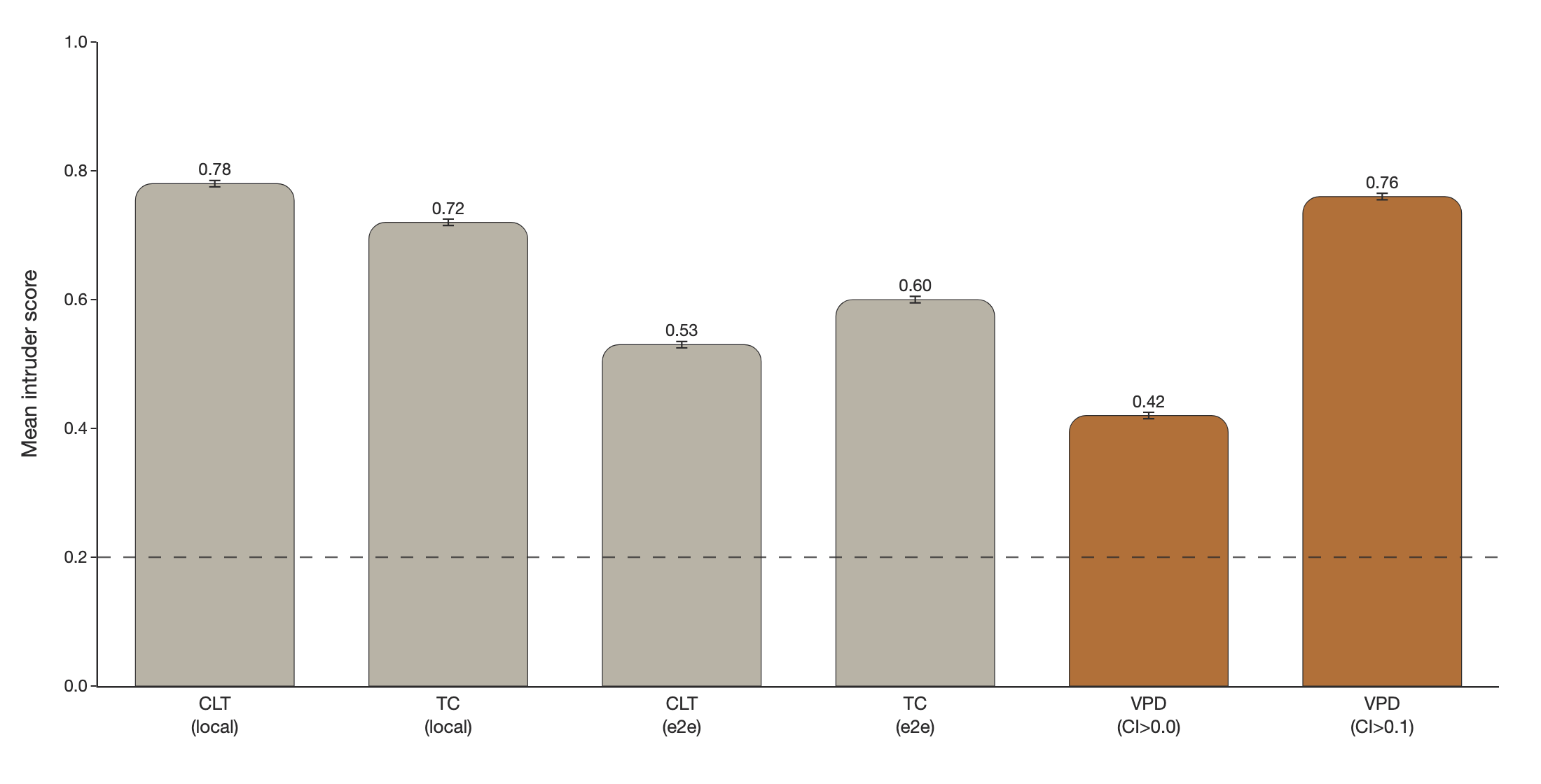
To compare how 'interpretable' parameter subcomponents are relative to transcoder latents, we can measure how semantically coherent a subcomponent's activation patterns are using *intruder detection* chang2009reading, paulo2025evaluating. In intruder detection, we present an LLM-judge with a set of inputs that activate a given VPD subcomponent or transcoder latent alongside one 'intruder' example that does not activate it. We task the LLM-judge to identify the intruder example. It should be easier to identify the intruder among a more semantically coherent set of inputs. In the VPD setting, we use causal importance values in place of activation magnitudes and select intruder examples with similar activation densities.
We find VPD intruder detection scores improve drastically when using CI values thresholded with 0.1, which filters low-CI noise fig:intruder-score. We think that filtering out small causal importances is justifiable, since 0.1-rounded performance has essentially the same performance as 0.0-rounded performance, suggesting that very little performance is captured by subcomponents with small activations (tab:vpd-ce-compute-compar).
We observe that 0.1-rounded VPD subcomponents score competitively with CLTs and PLTs trained using a local (layerwise) MSE activation reconstruction loss fig:intruder-score. VPD subcomponents are more coherent than PLTs and CLTs that were trained end-to-end.
Intruder detection scores for various CLT and PLT latents, and VPD subcomponents at different CI thresholds. Error bars are 95% bootstrap CIs on the mean. Dashed line is random chance accuracy (20%). Higher is better.
### VPD does not suffer from feature splitting {toc: No feature splitting}
Feature splitting is a well-known issue in activation-based dictionary learning methods such as PLTs, SAEs, and CLTs chanin2024absorptionstudyingfeaturesplitting, bricken2023monosemanticity. As dictionary size increases, these methods can improve sparsity and reconstruction by replacing a 'broad', reusable latent with several narrower, more context-specific ones. In the extreme, a transcoder could assign a unique latent to every individual datapoint in the training set, effectively memorizing the dataset rather than uncovering reusable, general patterns.
VPD does not suffer from this issue, either in principle or in practice. The key reason for this is that subcomponents marked as causally unimportant are required to be ablatable in any combination, not just all simultaneously. The model therefore needs to be robust to variations in parameter space along the directions of these subcomponents for all batches and sequence positions, not just the ones on which they are causally important. Without this constraint, the decomposition might be able to invent overly 'narrow', context-specific subcomponents that do not actually exist in the computational structure of the original model but that sparsely activate while reconstructing the model's behavior on some narrow subset of the data. For example, suppose VPD attempted to pathologically decrease $\mathcal{L}_{\text{importance-minimality}}$ by splitting a mechanism in the target model that ought to be parametrised by two subcomponents into many specialised subcomponents that lie within that mechanisms' two-dimensional subspace, each aligned with a different training-data hidden activation vector, and marked only one of them at a time as causally important. If we were just using the causal importances as masks, this would reconstruct the target model's output well. But with stochastic or adversarial masking, many of the subcomponents not marked as causally important will be turned on as well, making the resulting output activation vector both too large and pointed in the wrong direction, thus ruining the reconstruction. See sec:vpd_recon_motivation for further discussion.
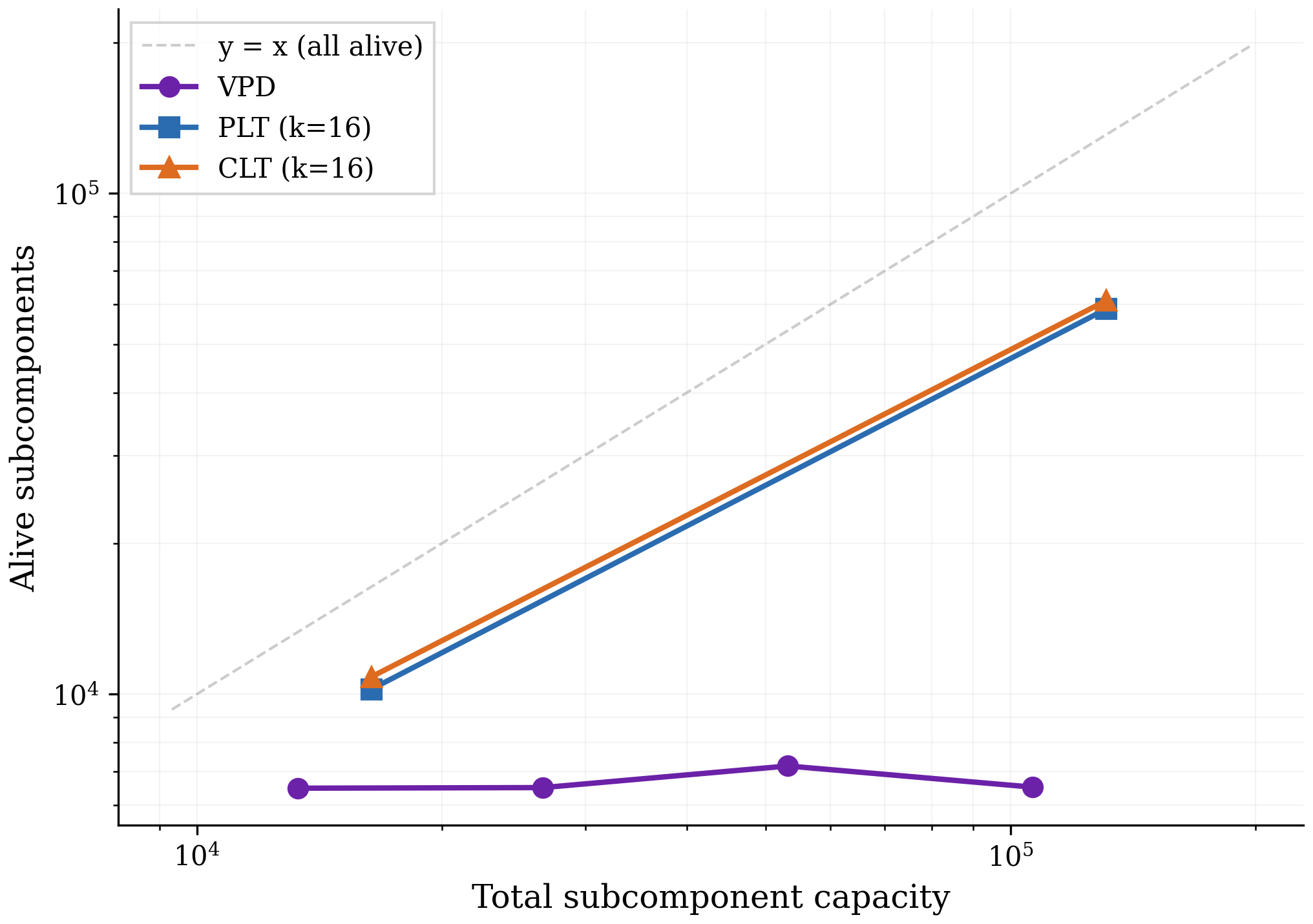
To test empirically whether VPD does avoid feature splitting, we incrementally increase the number of subcomponents used by different VPD runs and count the number of "alive" subcomponents (subcomponents that activate at least once every 1M tokens). We train VPD at four capacity levels corresponding to $0.5\times$, $1\times$, $2\times$, $4\times$ the subcomponent count of the main decomposition we study. We compare against PLTs and CLTs at 4k and 32k dictionary sizes.
Number of alive subcomponents as a function of total subcomponent capacity. PLTs and CLTs scale roughly linearly with dictionary size, staying close to the $y = x$ line. VPD (purple) remains flat at ~6,500-7,000 alive subcomponents regardless of capacity, indicating that additional capacity is not used for feature splitting. Dashed line: $y = x$ (all subcomponents alive).fig:feature_splitting shows that, unlike PLTs and CLTs, increasing VPD's capacity does not increase the number of subcomponents that the method actually uses, suggesting that feature splitting is not a significant problem for VPD. Across all four VPD runs the sparsity and reconstruction performance remain approximately constant, so the flat alive count reflects unused capacity rather than a tradeoff against sparsity or reconstruction. In app:confirming-feature-splitting, we confirm that our PLTs and CLTs are indeed splitting features rather than discovering genuinely new ones.
While we only show results for one language model here, we have observed the same qualitative result in every model we have decomposed with either VPD or SPD bushnaq2025spd despite extensive hyperparameter sweeps, including various toy models with known ground truth and a smaller language model trained on the SimpleStories (finke2025parameterizedsynthetictextgeneration) dataset.
## Decomposing attention behaviors that are distributed across attention heads {toc: Decomposing attention}
Transformer language models are significant in large part because they were the first architecture that enabled scalable sequence modelling. The crucial component that lets transformers perform computations across sequences is the attention layer (vaswani2017attention, Bahdanauetal2014).
In most prior work that studies attention layer computations, attention heads have typically been the primary units of analysis to study attention behaviors vig2019multiscalevis, clark2019doesbertlookat, elhage2021mathematical, olsson2022incontextlearninginductionheads, wang2022interpretability, janiak2023polysemantic, nam2025causalheadgatingframework. Unfortunately for interpretability, it is possible for attention layers to perform computations in a way that is distributed across multiple heads jermyn2023attention, jermyn2025attentionThis phenomenon is sometimes called 'attention head superposition'. However, we prefer to reserve that term for the specific case where the attention layer implements more computations than the number of heads it distributes them across, which might not happen in general.. It would therefore be ideal if our decomposition methods could cope with attention computations that are distributed across heads. So far, it has been difficult to find satisfactory activation-based decomposition methods that can do this jermyn2025attention, mathwin2024gated, wynroe2024qkbilinear, Kissane_Conmy_Nanda_2024, kamath2025tracing.
Fortunately, parameter decomposition methods offer some hope: As we've seen in sec:param-comps-interpretable, parameter subcomponents seem to decompose the parameters into specialized functional units. And since parameter subcomponents are vectors in parameter space, they can therefore span multiple attention heads!
In this section, we demonstrate that parameter subcomponents in attention layers are indeed interpretable, and can span multiple attention heads (and usually do!). Focusing primarily on attention layer 1, we study three attention layer behaviors ('*Previous token behavior*', '*Previous syntactic boundary movement*', and '*Detecting Existential vs. Expletive Constructions*') and show how parameter subcomponents distribute these computations across heads.
### Attention layer parameter subcomponents have specific interpretable roles {toc: Subcomponents have interpretable roles}
First, we look at a few parameter subcomponents in attention layer 1. In this layer VPD identifies different numbers of parameter subcomponents in the $W_Q$, $W_K$, $W_V$, and $W_O$ matrices. These matrices have 15, 48, 226, and 97 aliveThese subcomponent numbers correspond to the number of components with mean causal importance above $10^{-6}$. components respectively, though we'll usually present fewer for simplicity.
There are many interesting subcomponents in these matrices that correspond to easily interpretable behaviors:
- 1.attn.q:308 activates on tokens related to existence or the verb 'to be' and other 'copula' verbs.
- 1.attn.k:485 activates on words that predict 'copula' verbs, such as `·there` or `·it` in "there is/it is".
- 1.attn.k:218 activates on the word `·it` (including capitalized variations and variants both with and without a leading space)
- 1.attn.k:119 activates on punctuation, spaces, brackets, newlines and other 'interstitial' words.
- 1.attn.k:290 activates on newlines and end-of-text tokens only.
- 1.attn.v:42 activates on coordinating conjunctions, like `·and`, `·or`, `·but` and `·&`.
- 1.attn.v:178 activates on words related to position in time and, to a lesser extent, space, like `·December`, `·South`, `·2002`, `·long` and `·far`.
- 1.attn.o:983 Activates on the introductions or titles of texts, particularly scientific papers.
Additionally, there are some subcomponents whose role seems more related to 'sequence position' than having a particular semantic meaning:
- 1.attn.q:149 and 1.attn.q:497 tend to activate on the tokens immediately following the first token of the sequence (and, incidentally, reveal some of the shortcomings of our autointerp labelling method, which seems to have missed this!).
- 1.attn.k:315, 1.attn.k:357 and 1.attn.k:121 tend only to be causally important on the first few tokens of a sequence, though with some exceptions.
Together, these interpretations are encouraging, because they suggest that our decomposition is identifying parts of the network that are specialized for particular functional roles.
### Attention layer parameter subcomponents typically span multiple heads {toc: Subcomponents span multiple heads}
We've seen evidence that attention subcomponents are specialized for specific semantic roles, suggesting different computational functions. Now we investigate whether these subcomponents are 'located' in particular heads.
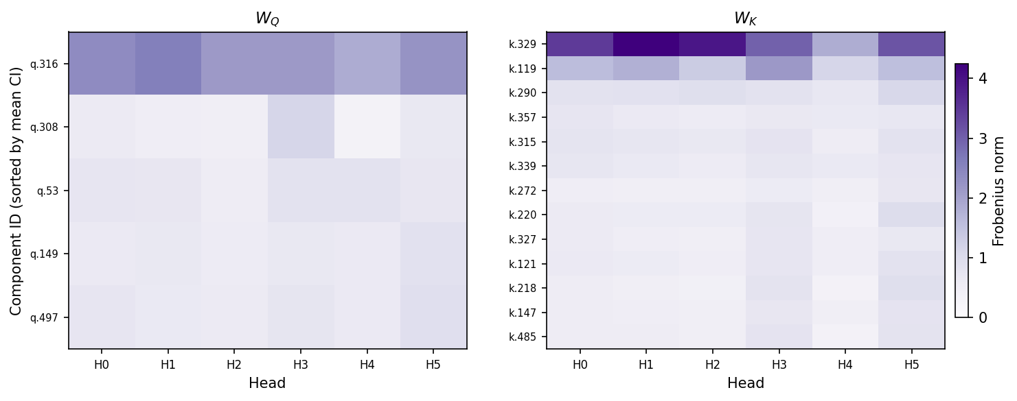
In our model, the $W_Q$, $W_K$, $W_V$, and $W_O$ matrices are concatenated across attention heads. But we can easily split them into the matrices belonging to individual heads. Even though parameter subcomponents by default span all heads in a layer, most of their 'mass' could be localized in single heads if their weights in all but one attention heads have zero norm. But if their parameters have nonzero norm in multiple heads, then this is weak evidence that they perform computations across multiple heads.
We'll focus on the $W_Q$ and $W_K$ matrices for now. We see that, in fact, most $W_Q$ and $W_K$ subcomponents have nonzero weight norm across each head (fig:qk_comp_weight_norm). This suggests that most $W_Q$ and $W_K$ subcomponents might perform computations in a distributed way! The norms subcomponents of $W_V$ and $W_O$ matrices seem similarly distributed across heads (fig:vo_comp_weight_norm)
The norm of the weights of each $W_Q$ and $W_K$ subcomponent in each head. No parameter subcomponent is exclusively localized in a single head, suggestive of computations that are distributed across attention heads.
While suggestive, this is only indirect evidence of distributed computations. We would need to understand the computations in order to confirm that they are indeed distributed across heads. To do this, we will need new analysis tools. And we can make the problem slightly easier by separately studying the two main parts of the attention layer: The QK circuit and the OV circuit elhage2021mathematical. We'll focus on the QK circuit first.
### The QK circuit consists of interactions between pairs of parameter subcomponents {toc: The QK circuit}
In attention layers, $W_Q\in \mathbb{R}^{d_{\text{model}}\times d_{\text{model}}}$ and $W_K\in \mathbb{R}^{d_{\text{model}}\times d_{\text{model}}}$ matrices transform sequences of activations $\varphi\in \mathbb{R}^{T\times d_{\text{model}} }$ in the (normed) residual stream to create queries ($q = \varphi (W_Q)^\top $) and keys ($k = \varphi (W_K)^\top$) for all heads. We can split them into the keys and queries for each head (e.g. $q = [ \varphi (W_Q^{1})^\top, \cdots , \varphi (W_Q^{H})^\top]$).
The attention scores of head $h$ are calculated as $Z^h = \varphi W_Q^{h \top} W_K^h \varphi^\top$, which are used to calculate the head's attention pattern, $A^h = \text{softmax} (Z^h) $.
Although the $W_Q$ and $W_K$ matrices are usually represented as separate matrices, it is convenient to study them together as a single matrix, $W_{QK}^h = W_Q^{h \top} W_K^h$ elhage2021mathematical.
Prior to parameter decomposition, it was not obvious how best to further decompose this circuit into specialized functional units. But VPD decomposes the $W_Q$ and $W_K$ matrices in a sum of functionally specialized rank-one parameter subcomponents The $V$ matrices of the subcomponents do not need $h$ indices because they only read from the residual stream. The $U$ matrices project into query or key space, and hence need $h$ indices.:
$$
W_Q^h = \sum_c \vec{U}^{h}_{Q,c} (\vec{V}_{Q,c})^\top \qquad \qquad W_K^h = \sum_c \vec{U}^{h}_{K,c} (\vec{V}_{K,c})^\top
$$
These subcomponents are secretly also a decomposition of the QK circuit, constructed from pairs of subcomponents of the $W_Q$ and $W_K$ matrices:
$$
\begin{aligned}
W_{QK}^h &= W_Q^{h \top} W_K^h \\
&= \left( \sum_c \vec{U}^{h}_{Q,c} (\vec{V}_{Q,c})^\top \right)^\top \left( \sum_{c'} \vec{U}_{K,c'}^{h} (\vec{V}_{K,c'})^\top \right) \\
&= \sum_{c, c'} \vec{V}_{Q,c} \left( (\vec{U}_{Q,c}^{h})^\top \vec{U}_{K,c'}^h \right) (\vec{V}_{K,c'})^{\top}
\end{aligned}
$$
We will use this equation to study the QK circuit, both for a form of static (*data-independent*) and dynamic (*data-dependent*) analysis of the computations of the QK circuit.
We'll need to define two new metrics, one to measure the static interaction strength between pairs of subcomponents and another to measure how strongly a pair of subcomponents are interacting on a particular datapoint.
#### QK Circuit - Metric 1: Static Interaction strength
Although we can use eq:qk-interactions to understand the *static interaction strength* between subcomponents $c$ and $c'$, we cannot simply use the raw term $\left( (\vec{U}_{Q,c}^{h})^\top \vec{U}_{K,c'}^h \right)$ for a few reasons:
First, because both $\vec{U}_c$ and $\vec{V}_c$ vectors are unnormalized, we need to scale each $\vec{U}_c$ vector by the norm of the corresponding $\vec{V}_c$ vector in order to put the $\vec{U}_c$ vectors on the same scale.
$$
||\vec{V}_{Q,c}|| \left( (\vec{U}_{Q,c}^{h})^\top \vec{U}_{K,c'}^h \right) ||\vec{V}_{K,c'}||
$$
Second, we need to incorporate sequence position information. The above equations actually leave out an important part of our transformer language model: The Rotary Position Embedding (RoPE) rotation matrix su2024roformer. For transformers that use RoPE, the QK circuit is actually: $W_{QK, \tau}^h = (W_Q^{h})^\top \boldsymbol{R}_{\tau} W_K^h$, where $\tau$ is the *offset*—the difference between the sequence position of the query and the key. The rotation matrix rotates the keys and queries by different amounts depending on the offset. Thus we have
$$
\left( ||\vec{V}_{Q,c}|| \vec{U}_{Q,c}^{h} \right)^\top \boldsymbol{R}_{\tau} \left( \vec{U}_{K,c'}^h ||\vec{V}_{K,c'}|| \right)
$$
Third, and finally, we need to know whether this interaction typically contributes positively or negatively to the attention score. To calculate this, we cheat slightly and import one data-dependent statistic: The sign of the average subcomponent activation for each subcomponent on tokens where the subcomponent is causally important. With these three adjustments, we get the Static Interaction Strength:
```equation
tex:
\htmlClass{hc-ac}{\text{StaticInteractionStrength}(c, c', \tau, h)}
\\ =
\htmlClass{hc-uq}{
\Big(
\htmlClass{hc-sign-q}{\text{sign}\left(\mathbb{E}_\varphi^{(c)} \left[\varphi\vec{V}_{Q,c} \right]\right)}
\htmlClass{hc-mag-q}{\lVert \vec{V}_{Q,c} \rVert}
\htmlClass{hc-uq-vec}{\vec{U}^h_{Q,c}}
\Big)^\top
}
\htmlClass{hc-r-tau}{ \boldsymbol{R}_{\tau} }
\htmlClass{hc-uk}{
\Big(
\htmlClass{hc-sign-k}{\text{sign}\left(\mathbb{E}_\varphi^{(c')} \left[\varphi \vec{V}_{K,c'}\right]\right)}
\htmlClass{hc-mag-k}{\lVert \vec{V}_{K,c'} \rVert}
\htmlClass{hc-uk-vec}{\vec{U}^h_{K,c'}}
\Big)
}
tips:
- hc-ac: The static interaction strength between subcomponent c and c' at offset τ in head h
- hc-uq: The transposed, scaled, signed left-hand vector of subcomponent c in the Q projection matrix of head h
- hc-sign-q: The sign of the average subcomponent activation of subcomponent c on a dataset of tokens where subcomponent c is causally important
- hc-mag-q: The magnitude of the right-hand vector of subcomponent c in the Q projection matrix
- hc-uq-vec: The left-hand vector of subcomponent c in the Q projection matrix of head h
- hc-r-tau: The RoPE rotation matrix at offset τ
- hc-uk: The transposed, scaled, signed left-hand vector of subcomponent c' in the K projection matrix of head h
- hc-sign-k: The sign of the average subcomponent activation of subcomponent c' on a dataset of tokens where subcomponent c' is causally important
- hc-mag-k: The magnitude of the right-hand vector of subcomponent c' in the K projection matrix
- hc-uk-vec: The left-hand vector of subcomponent c' in the K projection matrix of head h
```
The Static Interaction Strength metric is not directly comparable across heads, since each head applies a separate softmax function, making any differences in scales or averages of interaction strength irrelevant. To make the metric comparable across heads, we standardize it:
$$\text{StandardizedStaticInteractionStrength}(c, c', \tau, h) \\ = \frac{\text{StaticInteractionStrength}(c, c', \tau, h) - \mu_h}{\sigma_h}$$
where $\mu_h$ and $\sigma_h$ are the mean and standard deviation of the Static Interaction Strengths across all $(c, c', \tau)$ for head $h$.
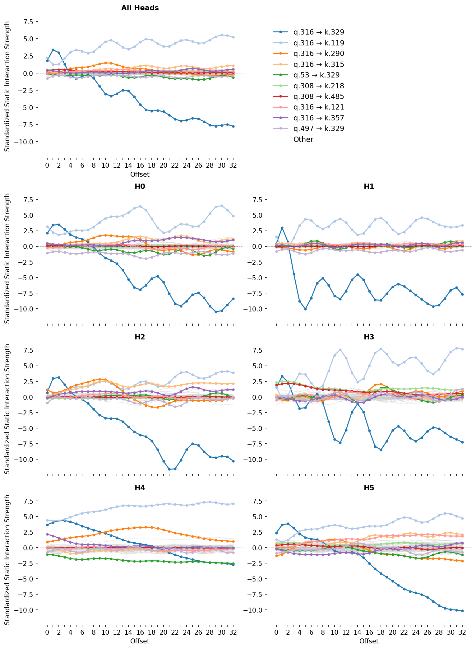
For attention layer 1, we plot this metric for each pair of subcomponents for each head and offset (fig:attn_contrib_grid). We can see that for some pairs, the Static Interaction Strength changes strongly at different offsets. This means that, for these pairs, the same activations might have different effects on the attention at different offsets! For others, the Static Interaction Strengths seem independent of offset, meaning that their effects on the attention scores are determined only by whether data that activate them are present.
The Standardized Static Interaction Strengths of pairs of parameter subcomponents in the $Q$ and $K$ projection matrices in each head (bottom grid) and all heads (top). The ten pairs with the largest interaction strengths at any offset are shown in color, with the rest in grey. The 1.attn.q:316 and 1.attn.k:329 pair exhibit strong positive Static Interaction Strength at early offsets, indicating this pair's involvement in cross-head previous token behavior (and, more generally, 'recent token behavior'.
We will use this plot of Static Interaction Strength to analyze particular attention behaviors. But before we do, we will equip ourselves with a related metric, the Data-Dependent Interaction Strength, which permits dynamic analysis.
#### QK Circuit - Metric 2: Data-Dependent Interaction Strength
The attention patterns of each head depend on how the hidden activations interact with the QK circuit: $A^h_\tau = \text{softmax} (\varphi W_{QK, \tau}^{h} \varphi^\top)$.
We can use eq:qk-interactions to decompose the QK circuit and study how the activations $\varphi$ at different timesteps $t,t'$ interact with each of the pairs of subcomponents:
$$
\begin{aligned}
Z^h_\tau &= \varphi W_{QK, \tau}^h \varphi^\top
&= \sum_{c, c'} \varphi \vec{V}_{Q,c} \left( (\vec{U}^{h}_{Q,c})^\top \boldsymbol{R}_{\tau} \vec{U}^h_{K,c'} \right) (\vec{V}_{K,c'})^{\top} \varphi^\top
\end{aligned}
$$
Thus, the attention score at each head $h$ and offset $\tau$ consists of the sum of the data's interaction with each of the individual pairs $(c, c')$. On any input, we can therefore decompose the attention score—and hence the attention pattern—into parts that we can study in isolation. This lets us define a data-dependent metric of interaction strength, which forms the basis of our dynamic analysis:
$$
\begin{aligned}
\text{DataDependentInteractionStrength}(c, c', \tau, t, t', h)
&= \left(\varphi \vec{V}_{Q,c} \left( (\vec{U}^h_{Q,c})^\top \boldsymbol{R}_{\tau} \vec{U}^h_{K,c'} \right) (\vec{V}_{K,c'})^{\top} \varphi^\top\right)_{t,t'}
\end{aligned}
$$
If we broadcast this over sequence position and head, we can visualise a subcomponent pair's interactions across a whole prompt as a stack of per-head matrices — and the model's full attention score $Z$ as the (per-head, per-position) sum of every such pair. To keep the figure readable, we'll abbreviate the position-independent pair term as
$$
\text{DataDependentInteractionStrength}(c, c', :, t, t') := \left( \varphi \vec{V}_{Q,c} \left( (\vec{U}_{Q,c})^\top \vec{U}_{K,c'} \right) (\vec{V}_{K,c'})^{\top} \varphi^\top\right)_{t,t'},
$$
```attention-equation
data: data/attention/intro-layer-1.json
caption: Attention scores $Z$ illustrated as a sum of Data Dependent Interaction Strengths between pairs of subcomponents.
```
In fig:dynamic-1, you can select which subcomponent interactions to sum together and see the attention score for those pairs. This is a very useful tool, since it splits up any given attention pattern into the contributions of individual, functionally distinct, subcomponent interactions.
```attention-cards
label: fig:dynamic-1
data: data/attention/intro-layer-1.json
caption: The attention score consists of a sum of Data Dependent Interaction Strengths. This panel shows the same prompt as the figure above, but here you can control which pairs of subcomponents to include in the sum, allowing you to study their individual effects on the reconstructed attention score and attention pattern.
```
We'll do an initial analysis of an attention behavior using only these two QK metrics before discussing how they interact with the OV circuit.
### Decomposing attention behavior 1: Previous token behavior {toc: Behavior 1 - Previous token behavior}
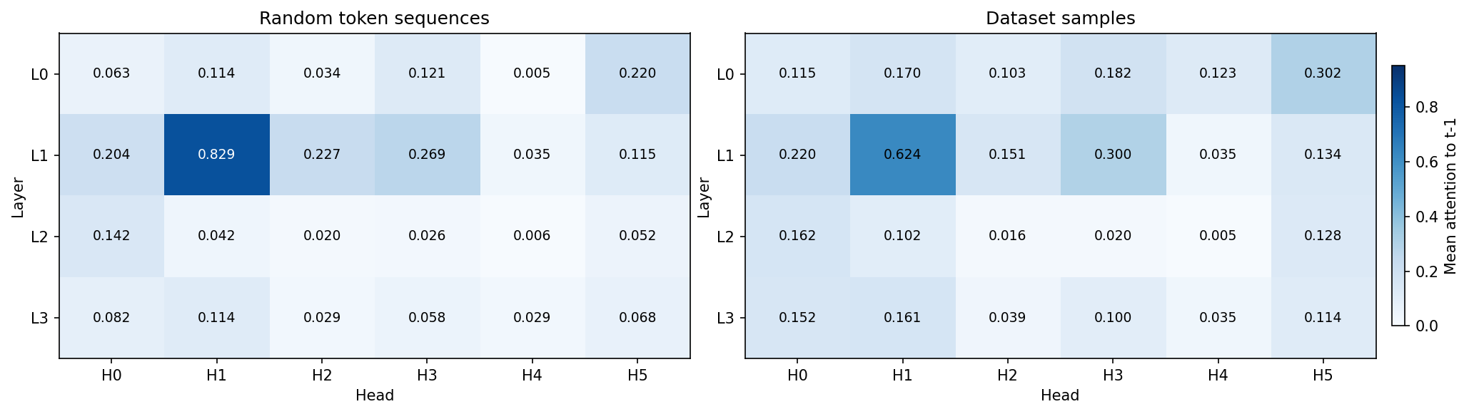
Like many language models, our model has a head that, on average, places the majority of its attention on the previous timestep (fig:prev_token_scores). This is typically called a *previous token head* clark-etal-2019-bert,elhage2021mathematical, olsson2022incontextlearninginductionheads, wang2022interpretability and, in our model, is head 1 in layer 1 (**L1H1**). However, L1H1 is not the only head to assign substantial probability to the previous token; many other heads do too, including heads in the same layer as L1H1.
Identifying the previous token head: Mean attention across multiple inputs on offset $\tau=1$, i.e. the previous token.
**Left**: Average over sequences of random tokens, as per wang2022interpretability. **Right**: Average over sequences sampled from the dataset. The plots reveal L1H1 is the most canonical "previous token head". But note other heads place substantial average attention at offset $\tau=1$.
Now we need to find subcomponents that might be involved in previous token behavior and establish whether or not their computations span multiple heads. An obvious place to start is by looking at the largest, most frequently active subcomponents in the $W_Q$ and $W_K$ matrices. Perhaps by coincidence, the largest norm subcomponents, 1.attn.q:316 and 1.attn.k:329, are also the most frequently causally important (fig:qk_comp_weight_norm)!
While most subcomponents in layer one are only active on a fraction of tokens, both 1.attn.q:316 and 1.attn.k:329 have a CI firing density of $96.7\%$ and $99.8\%$, meaning they're nearly constantly active. Both have the largest weight norm in L1H1, which was the head with the strongest previous token behavior (fig:qk_comp_weight_norm). But they also have substantial weight norm in other heads, suggesting they aren't exclusively located in any particular head. Could they be responsible for cross-head previous token behavior?
fig:attn_contrib_grid shows that these two subcomponents also have very strong offset-dependent Static Interaction Strength. In particular, their interaction is strongest at small offsets, and weak or negative interactions at more distant offsets. This is exactly what we would expect of two subcomponents that implement previous token behavior or recent token behavior. This pattern holds not only in L1H1, but also in other heads too. This is strong observational evidence that these two subcomponents compute previous token behavior in a way that is distributed across heads.
We test this hypothesis causally using ablations and dynamic analysis. When we ablate different $W_Q$ subcomponents on a dataset of prompts, the change in average attention is very small for most subcomponent ablations. Only the ablation of 1.attn.q:316 results in the large reduction of attention at recent offsets (fig:attn_patterns_q_intv).
Effect of ablations: Ablating 1.attn.q:316 very strongly reduces attention to tokens in the recent past across all heads that otherwise attended there strongly. The effects of ablating other W_Q components has no distinguishable effect compared with the baseline and are therefore not shown. Here the baseline is the unablated average attention pattern.fig:dynamic-1 shows dynamic analysis. For any of the prompts, you can remove the contribution of the 1.attn.q:316 and 1.attn.k:329 interaction to the attention score. Removing it destroys the attention to tokens in the recent past across all heads that had strong to moderate attention there.
Together, this is strong evidence that the 1.attn.q:316 and 1.attn.k:329 interaction computes previous token behavior and is distributed across heads.
This raises a question: What information is this attention moving from the recent past to the current timestep? What *attention values* does this previous token behavior tend to move? Are the different heads carrying forward information from distinct subspaces in the residual stream? Or are they carrying redundant information, perhaps as a form of noise robustness? To study this, we need to analyze the OV circuit, for which we will need another metric.
#### Previous token behavior employs non-overlapping subspaces in the OV circuit
The OV circuit is made from the $W_V$ and $W_O$ matrices which respectively read from and write to the residual stream:
$$
W_{OV}^h = W_{O}^h W_{V}^h \in \mathbb{R}^{d_{\text{model}} \times d_{\text{model}}}
$$
The sequence of $T$ vectors of dimension $d_{\text{model}}$ that the attention layer outputs into the residual stream is computed using the attention pattern-weighted sum of the outputs of the OV circuits at all previous timesteps (where the attention pattern $A^{h}$ is determined by the QK circuit):
$$
\text{AttentionLayer} (\varphi) = (A^h)^\top \varphi (W_{OV}^h)^\top \in \mathbb{R}^{T \times d_{\text{model}}}
$$
Although $W_{OV}^h$ is a $d_{\text{model}} \times d_{\text{model}}$ matrix, it only has rank $d_{\text{head}}$. Being low rank, each head can therefore only read from and write to a small subspace of the residual stream. It would be useful to know if two heads read from and write to similar subspaces.
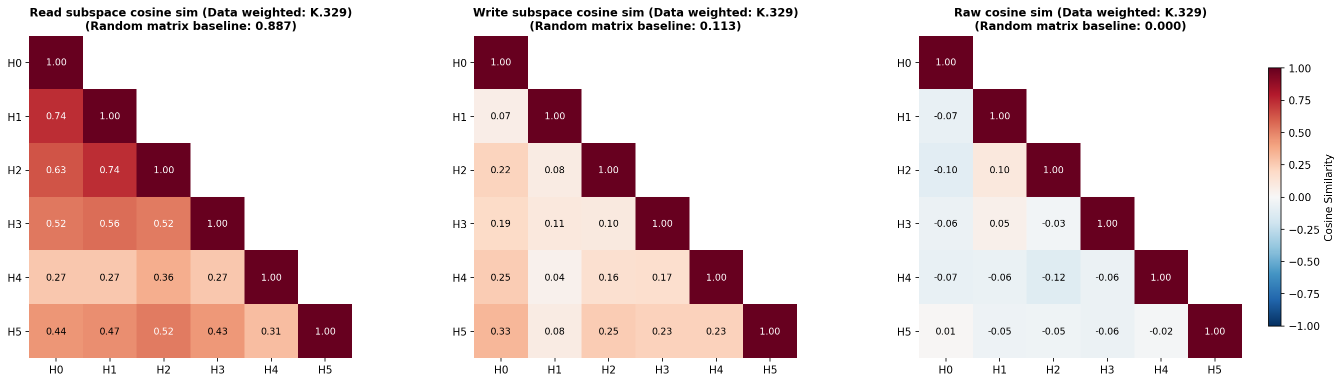
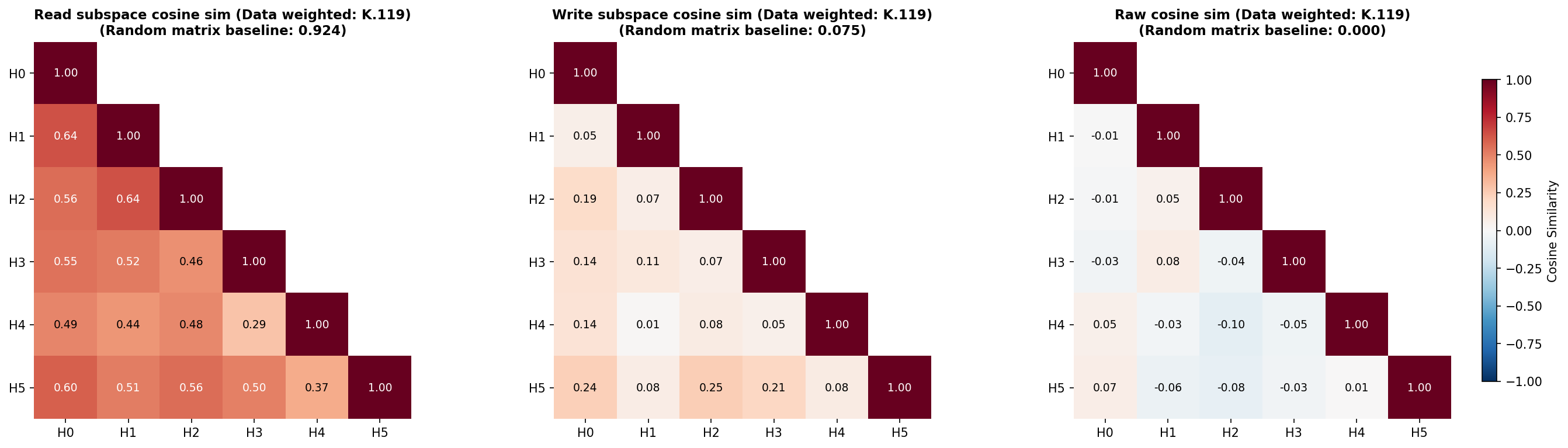
To do this, we will measure the 'overlap' between the subspaces that each head's OV circuit reads from and writes to, for which we'll use the 'Data-weighted Subspace Similarity' metric, which we construct from the Frobenius cosine similarity of the 'read subspaces' and the 'write subspaces' of each head (fig:prev_tok_ov_overlap_k_329). See app:OV-metric-data-frob for details of how these subspaces are constructed and for further details of this metric. We also measure the Frobenius cosine similarity of the $W_{OV}^h$ matrices themselves (fig:prev_tok_ov_overlap_k_329). When calculating similarity, we weight the axes of the read- and write-subspaces by how much data variation lies in each axis, since we do not care as much about weight similarity along axes where data do not exist or do not vary. In all cases, we compare the measured similarities to similarities between random, data-weighted matrices.
Most heads in layer 1, except L1H4, seem at least weakly involved with previous token behavior, as assessed by their previous token score (fig:prev_token_scores) and the offset dependence of the Static Interaction Strength of the 1.attn.q:316 and 1.attn.k:329 pair (fig:attn_contrib_grid). We therefore should look at the overlap in the read and write subspaces of all heads in layer 1 except L1H4.
The read subspaces of each head are close to or slightly lower than the expected similarity of two random (data-weighted) matrices (fig:prev_tok_ov_overlap_k_329). On the other hand, the write subspaces seem close to or slightly higher than the random baseline. These effects seem very weak, but weakly suggest a pattern of attention heads reading from distinct subspaces but writing to slightly less distinct subspaces.
Data-weighted cosine similarities between each head's $W_{OV}^h$ read and write matrices, and the cosine similarity between each head's raw $W_{OV}^h$. Here, data-weighting uses data where subcomponent 1.attn.k:329 is causally important.
For the head with the strongest previous token behavior, L1H1, the other heads L1H0 and L1H2 seem to read from subspaces with similarities close to the random baseline, but other heads read from much less similar subspaces. When comparing the similarity of the raw $W_{OV}^h$ matrices, there appears to be very little deviation from levels of overlap that would be expected of random matrices, except the comparison between L1H1 and L1H2, which again seem to be more similar than the random baseline. These two heads seem to write to quite different subspaces, though.
Overall, this weakly suggests a picture that previous token behavior spans distinct subspaces across different heads. One potential reason for this is to be able to read more information from the residual stream than might be readable by a single head. There appears to be very limited, but nonzero, redundancy in how heads involved in previous token behavior read from different subspaces, but they largely seem to write to different subspaces.
Previous token behavior is an important behavior implemented by probably every language model. But it is far from the only behavior implemented in layer 1. Even in L1H1, only around 60% of attention is on the previous timestep (fig:prev_token_scores). What other attention behaviors is this head implementing? In the next section, we look at another behavior implemented by L1H1 in more detail, and examine whether that behavior is also distributed across heads.
### Decomposing attention behavior 2: Previous syntax boundary movement {toc: Behavior 2 - Previous syntactic boundary movement}
Looking again at the static analysis of layer 1, we can see that L1H1 has interactions between Q and K subcomponents that seem to have quite a different offset-dependency (fig:attn_contrib_grid). The subcomponents 1.attn.q:316 and 1.attn.k:119 seem to interact most strongly at later offsets across multiple heads, including L1H1.
We are already familiar with 1.attn.q:316, the query subcomponent that is always active. The key subcomponent 1.attn.k:119 is new: It seems to activate on brackets, punctuation, and newlines, but also some common continuation words, such as 'the' or 'and'. It is causally important on 16% of tokens, which is frequent, but not constantly active.
This interaction therefore involves a conditional computation: Although 1.attn.q:316 is always active, constantly looking back in time, the other subcomponent 1.attn.k:119 only interacts with it when it is active.
Interestingly, 1.attn.k:119 must be active sufficiently far back in time; otherwise, the Static Interaction Strength may not be strong enough to contribute to the attention score. Almost every head seems to exhibit an offset dependent interaction between subcomponents 1.attn.q:316 and 1.attn.k:119, suggestive of a very distributed computation.
Since this computation is data-dependent, we will benefit from greater use of dynamic analysis. fig:dynamic-2 shows the attention patterns of all heads, but only shows the Data Dependent Interaction Strength of the 1.attn.k:119-1.attn.q:316 interaction. One prompt is shown at a time, but you can select a variety of other prompts from the dataset in the dropdown menu.
```attention-cards-solo
label: fig:dynamic-2
data: data/attention/30-dataset-layer-1.json
q_comp: 316
k_comp: 119
caption: Data Dependent Interaction Strength for the 1.attn.k:119-1.attn.q:316 interaction only, and the corresponding attention pattern if only that interaction contributed to the attention pattern. On the right hand side, the ground truth attention pattern is shown for comparison.
```
By exploring different prompts, and inspecting the contributions of the 1.attn.q:316 and 1.attn.k:119 interaction across all heads, it is possible to see that this interaction contributes significantly to the attention patterns of most heads on previous periods, commas, and newline characters. L1H4 seems capable of maintaining attention on these characters at quite large offsets, based on the stronger than average vertical bars in the ground truth attention on those tokens. Other heads seem only to have noticeable attention on them more recently in time. This may be due to competition with other attention score contributions from other pairs.
The activating examples of 1.attn.k:119 show firings on various forms of punctuation, end of text tokens, newlines, latex "$" symbols, brackets, etc. This suggests that this pair of subcomponents orchestrates a syntax boundary detector with a variety of short- or long-offset ranges. We'll call this 'previous syntax boundary' movement.
This pair of subcomponents seems responsible for attention to syntax boundary tokens at different ranges in different heads (fig:attn_contrib_grid). L1H1 seems to increase self attention upon syntax boundary tokens; L1H2 seems only mildly to attend to syntax boundary tokens and only in the very recent past. L1H5 and L1H0 attend to syntax boundary tokens a small number of tokens in the past. L1H4 seems to attend to syntax boundary tokens many tokens in the past. L1H3 is less clear, but seems to attend to a smaller subset of specific syntax boundary tokens, usually with shorter offset ranges.
The QK circuit of the 'previous syntax boundary movement' behavior seems quite distributed across heads. How does it interact with the OV circuit? We can study this by looking at probability of each key subcomponent being active conditioned on a given value subcomponent being active (fig:pkv). The value subcomponents most associated with 1.attn.k:119 are:
- 1.attn.v:72
- 1.attn.v:22
- 1.attn.v:745
- 1.attn.v:919
- 1.attn.v:531
- 1.attn.v:494
- 1.attn.v:195
- 1.attn.v:612
- 1.attn.v:984
- 1.attn.v:1000
- 1.attn.v:22
- 1.attn.v:389
- 1.attn.v:188
- 1.attn.v:299
- 1.attn.v:1014
- 1.attn.v:227
- 1.attn.v:946
- 1.attn.v:340
- And some with weaker associations (fig:pkv).
As in the case of previous token behavior, the data-weighted OV circuits (where we weight the similarity using dataset examples and tokens where 1.attn.k:119 is causally important) do not seem to read from very similar residual stream subspaces (fig:prev_tok_ov_overlap_k_119), though they seem to write to somewhat more similar subspaces than would be expected in random matrices. The OV circuit subcomponents that subcomponent 1.attn.k:119 seems to overlap strongest with are associated with other punctuation and syntax boundary-like tokens across seemingly all heads, in both the read and the write matrices (app:ov-alignment-k119).
To understand why the model is carrying forward information about the previous syntax boundary, we would need to know how the values are being used downstream. But it is possible to surmise at least part of its function: It is useful to know what the previous syntax boundary tokens are in order to perform tasks like closing opened brackets; knowing whether a list is a bullet list or dashed list; or knowing if a token is within or outside of a quotation; and more.
### Decomposing attention behavior 3: Detecting Existential vs. Expletive Constructions {toc: Behavior 3 - Detecting Existential vs. Expletive Constructions}
Both of the above attention behaviors (sec:attn-analysis-1 and sec:attn-analysis-2) have involved $W_Q$ or $W_K$ subcomponents where one is 'always active'. Although the vast majority of the attention scores in this layer seem to involve at least one of these subcomponents, it would be interesting to study an even more conditional behavior.
We'll investigate an attention behavior involving the $W_Q$ subcomponent 1.attn.q:308.
This subcomponent appears to activate on a subset of **copula** verbs. Examples of copula verbs include:
- "To be" ("she **is**", "it **was**", "What **were**", ),
- Verbs related to sensory appearance ("it certainly **seems**", "she **appeared** as though", "they **looked** like"), and
- Verbs related to state ("we **remain**", "it **becomes** readily apparent", "there **exists**").
Grammatically, copula verbs behave as *linking verbs*: They connect a subject ("it", "she", "there", "we", etc.) to a description or complement, rather than expressing an action. They are relatively ubiquitous throughout English, so it makes sense that even a small language model would learn computations involving them.
#### Subcomponent 1.attn.q:308 activates on a subset of copula verbs
Although 1.attn.q:308 has a large subcomponent activation on copula verb tokens, it is noteworthy that it is not causally important on all instances them. Here are several prompts containing copula verb tokens on which 1.attn.q:308 is not causally important on some tokens despite having high subcomponent activation:
```prompt-viewer
data: data/manual-prompts/1-attn-q-308.json
```
By contrast, here are a few prompts where 1.attn.q:308 *is* causally important on copula verb tokens:
```prompt-viewer
data: data/manual-prompts/1-attn-q-308-important.json
```
By studying the difference between these two sets, it is possible to notice a pattern: Although 1.attn.q:308 has a large positive subcomponent activation on most instances of copula verbs, the cases where it is causally important are typically when it is preceded by `it`, `there`, `here` (as in "it is", "there is", "there are", "here is", "makes it seem") and related tokens.
Constructions like these have specific linguistic terms: **Existential** and **expletive constructions**, which use "there" and "it" in particular senses:
- The '**existential "there"**': Where "there" is used to make assertions about the existence of something. *Examples: "**There is** a problem", "**there wasn't** enough", "**there seems to be** several", "**there exists**", "**there have been** few attempts", "**there remains** a number of"*
- The '**expletive "it"**': Where "it" is used as a dummy subject, with no real referent. *Examples: "**It is** unusual", "**It appears** likely", "**It was** found that", "**It dawned** on him that"Note that, even though "dawned" is not a copula, we can still use the 'expletive "it"' with it., "**It looks** like"*
Even though 1.attn.q:308 has a high subcomponent activation on most copula verbs, it is usually not causally important (with some exceptions) when the copula verb is preceded by personal pronouns (e.g. "she", "he", "they"):
```prompt-viewer
data: data/manual-prompts/1-attn-q-308-personal-pronoun-copula.json
```
How could this be? The main way that QK subcomponents can influence downstream computations (and hence have causal importance) is by influencing attention. 1.attn.q:308 having a large subcomponent activation is insufficient for attention. There needs to be a key subcomponent that aligns with 1.attn.q:308 (i.e. has a high Static Interaction Strength) that also has a high subcomponent activation in order for a Q-K subcomponent pair to have high Data Dependent Interaction Strength, and hence to contribute significantly to the attention pattern. There must therefore be $W_K$ subcomponents that 1.attn.q:308 'looks for' in the past that, if present, give this subcomponent its causal importance.
#### Subcomponent 1.attn.q:308 interacts with two specific $W_K$ subcomponents
We'll start looking for this interaction by looking at whether there are subcomponents that have a high Static Interaction Strength with 1.attn.q:308.
Looking again at fig:attn_contrib_grid, we can see that 1.attn.q:308 has strongest offset-dependent Static Interaction Strength with two $W_K$ subcomponents, namely 1.attn.k:218 and 1.attn.k:485. These two interactions are strongest in L1H3, but also in L1H5.
Incidentally, the norm plot (fig:qk_comp_weight_norm) supports the idea that 1.attn.q:308 is primarily located in L1H3, and secondarily in L1H5, since the weight norm is largest in those two heads and negligible elsewhere.
These two $W_K$ subcomponents (1.attn.k:218 and 1.attn.k:485) seem to be causally important on related, but semantically distinct, tokens, which we explore in detail in the following sections.
#### Subcomponents 1.attn.k:218 and 1.attn.q:308 make an "it + copula verb" detector
1.attn.k:218 seems to have high subcomponent activation on any instance of the word "it", including capitalized variants. It is also causally important on any instance of the word "it", but its causal importance tends to be higher on instances of the 'expletive "it"'This includes edges cases like the 'meterological it', as in "It is raining.".
The phrase "it is" is often an 'expletive "it"' followed by a copula. But it may also be an 'anaphoric pronoun "it"' followed by a copula, as in "It is mine". It turns out that 1.attn.k:218 is causally important on both types of "it is". But it is not causally important for expressions involving other pronouns followed by copulas, such as "he is", "they are", etc. It therefore seems that this pair of subcomponents interact to implement an "it + copula verb" detector, including both 'expletive "it"' and 'anaphoric pronoun "it"' followed by a copula
We can see its Data Dependent Interaction Strengths in the figure below. The interaction strengths are strongest in L1H3, with a small amount in L1H5, with essentially none in any other head. The attention patterns reveal that the 1.attn.q:308 subcomponent 'looks back in time' from copula verbs, and has high Data-Dependent Interaction Strength with 1.attn.k:218 if it finds it. If it does, it usually contributes enough to the attention score that it becomes causally important.
```attention-qk-grid
data: data/attention/behavior-3/outputs/k-218-copula.json
q_comp: 308
k_comp: 218
```
It turns out that it is quite an overzealous "it + copula verb" detector. It often produces high Data Dependent Interaction Strength even at quite large offsets, even when the "it" and the copula verb are not related to each other. For an example, see the prompts below where a copula verb late in the prompt attends back to an unrelated ` it` token in an earlier sentence:
```attention-qk-grid
data: data/attention/behavior-3/outputs/k-218-overzealous.json
q_comp: 308
k_comp: 218
```
#### The 1.attn.k:485-1.attn.q:308 interaction plays a mostly overlapping role to the 1.attn.k:218-1.attn.q:308 interaction
The other subcomponent with which 1.attn.q:308 has a strong interaction is 1.attn.k:485. It has strongest subcomponent activation on the word "there", but also activates for "here" and "it" (and all their capitalized variants). It tends to be causally important when any of these words is followed by a copula verb.
```attention-qk-grid
data: data/attention/behavior-3/outputs/k-485-copula.json
q_comp: 308
k_comp: 485
```
Together, this indicates that the interaction between 1.attn.k:485 and 1.attn.q:308 causes attention to **existential constructions**, such as "There is", "Here are", "There exists", as well as **expletive constructions** (which we studied in detail in the previous subsection). This means that its function overlaps with the function of the 1.attn.k:218 and 1.attn.q:308 interaction, which also detects expletive constructions.
However, the 1.attn.k:485-1.attn.q:308 interaction contributes relatively less attention to expletive constructions compared with the interaction between 1.attn.k:218 and 1.attn.q:308. For example, in the prompt below, the 1.attn.k:485-1.attn.q:308 interaction misses the 'expletive "it"' in "make it probable" while 1.attn.k:218-1.attn.q:308 detects it and causes attention to it.
```attention-qk-grid
data: data/attention/behavior-3/outputs/compare-single.json
q_comp: 308
k_comp: 485
```
```attention-qk-grid
data: data/attention/behavior-3/outputs/compare-single.json
q_comp: 308
k_comp: 218
```
These two interactions thus both play overlapping, but somewhat specialized roles in detecting what type of construction a copula verb is in.
#### Both QK subcomponent interactions have similar OV circuits
Their overlapping, but slightly distinct, roles are reflected by their OV circuits.
If either 1.attn.k:218 and 1.attn.k:485 are causally important, the $W_V$ subcomponents with the highest probability of also being causally important are (fig:pkv):
- 1.attn.v:744
- 1.attn.v:180
- 1.attn.v:946
- 1.attn.v:649
However, both $W_K$ subcomponents do not have identical relationships with all $W_V$ subcomponents. Subcomponent 1.attn.v:448 seems only to have a high conditional probability of being causally important with 1.attn.k:485, not 1.attn.k:218. Combined, these values seem to be carrying both grammatical and 'content' information. It's worthwhile noting that these $W_V$ subcomponents are not localized to particular heads, and therefore their information may be mediated via more than one head (fig:vo_comp_weight_norm).
On a normative level, why does the model learn these two behaviors and implement them in this way? On one level, the answer is somewhat obvious: These constructions (existential, expletive, anaphoric) tend to be followed by different types of text, which therefore demands different kinds of predictions. On another level, it feels likely that a better model could have implemented better detectors. To determine whether layer 1 is simply too early in the model for a 'cleaner' implementation, or whether the model is simply too small, would require further investigation. We leave those investigations, as well as studies of how these overlapping, but separable, detectors influence downstream computations, to future work.
We have barely scratched the surface of the extent and complexity of attention computations of even this small model. Nonetheless, we are excited by the possibilities for understanding attention computations opened up by decomposing attention layer parameters into parameter subcomponents. We believe the breadth of this analysis could be massively increased and note there is significant room for increasing the depth analysis that use parameter subcomponents to decompose and understand attention. We have not, for instance, studied how parameter subcomponents could interact across attention layers, perhaps forming structures akin to 'virtual attention heads', but decomposed into their constituent parameter subcomponents.
## Interpreting circuits of parameter subcomponents {toc: Circuits}
So far, we have studied parameter subcomponents individually, or one attention layer at a time, looking at how they combine within a single attention layer to produce behaviors like previous-token movement and previous-syntactic-boundary movement. But the outputs of a language model are computed using many layers in series. In this section, we use parameter subcomponents to understand at least some aspects of the target model's internal computations from the input embedding all the way to the output on a few different prompts.
To make sense of these multi-step computations, we need a way to study how information flows between parameter subcomponents throughout the entire model. We do this by calculating attributions, which measure the strength of the interaction between causally important subcomponents on particular prompts. The resulting attribution graphs let us trace, on individual prompts, how information moves between subcomponents across layers. In particular, we use gradient attributions, but use stop-gradients on every node other than the source and target so that we measure only the 'direct' effects of one subcomponent on another (sec:attr-calcs).
It should be noted that using gradients in this way 'abstracts away' the complexity of non-linear interactions between subcomponents by summarizing them into a single number. As a result, such attributions are only 'local' measures of interaction strength; their value depends on the particular datapoint that we measure them on. Many works have pointed out issues (such as saturated softmax functions in attention layers) that can cause such local attributions to be unrepresentative of more 'global' measures kramár2024atpefficientscalablemethod, jafari2025relpfaithfulefficientcircuit. In order to identify more 'global' measures of interaction strength, we would need to better characterize the nonlinear relationships between parameter subcomponents. This is an important research priority, and one that we've already begun exploring, but not something that this paper covers in detail. We do nonetheless provide analysis that suggests parameter subcomponents of MLP matrices, despite not being directly selected to have simple interactions, tend toward it anyway (app:interactions-gis-vs-coact).
### Attribution calculations
To calculate attributions between two subcomponents, we leverage gradients. In particular, we calculate the gradients between each "subcomponent activation", $a^l_c = (\vec{V}^l_c)^\top \vec{\varphi}^l$. However, we do not always simply use $\frac{\partial a_{c}}{\partial a_{c'}}$, the partial derivative of the target subcomponent activation $a_{c}$ with respect to the source subcomponent activation. The partial derivative measures the influence of $a_{c'}$ on $a_{c}$ through both *direct* and *indirect* pathways. Understanding the direct effects of a subcomponent give us the clearest mechanistic picture of its role in the network's neural algorithm. We therefore need an attribution method that can distinguish between direct and indirect effects, unlike the partial derivative $\frac{\partial a_{c}}{\partial a_{c'}}$. But, complicating matters further, in models with residual streams a subcomponent's direct effects are not limited only to those in the immediate next layer. The direct effects may skip many layers!
Instead of using the partial derivative $\frac{\partial a_{c}}{\partial a_{c'}}$, we use the fact that we can control how gradients flow on the backwards pass. We take the partial derivative $\frac{\partial a_{c}}{\partial a_{c'}}$, but we stop the gradients flowing through all subcomponents that are not the source subcomponent (fig:attr-graph-expl). This avoids measuring their effects on the target node, including the indirect effects of the source node that flow through them.
To exclude indirect effects (i.e. effects that one parameter subcomponent has on another that are mediated by intermediate parameter subcomponents), we stop the gradients flowing through all subcomponents that are not the source subcomponent.
This derivative approximates how sensitive the target node is to the source node. Our attribution multiplies this "sensitivity" by the strength of the activation of the source node in order to measure its overall influence. Additionally, we do not want to include causally unimportant nodes in our attributions, and therefore multiply the resulting term by the source subcomponent's causal importance:
$$\text{attr}(c' \to c) = \left( \frac{\partial a_c}{\partial a_{c'}} \right)^* \cdot a_{c'} \cdot g_{c'}$$
where the $*$ around the partial derivative denotes stopped gradients on non-source subcomponents.
For more details on our gradient attributions, see app:gradient_attributions.
### Pruning for specific behaviors
Most prompts, even simple ones, tend to activate hundreds of parameter subcomponents, which is too many to analyze at once!
We can further reduce the number of subcomponents we need to analyze by keeping only those subcomponents involved in computing some particular output behavior on a prompt that we are interested in.
To do this, we use two types of pruning methods, yielding two types of attribution graph. We'll use both types in our analysis below:
- **Attribution graph type 1: Pruning with adversarial sampling**: Suppose, on the prompt `The` `·princess` `·lost` `·her` `·crown` `.`, we wanted to analyze how the model successfully predicts `·her`. We would therefore only be interested in subcomponents that were involved in computing this specific prediction at this specific sequence position, which is a smaller subset of subcomponents than the set used to predict all tokens at all sequence positions. We can therefore find *new* causal importances to identify only those subcomponents by minimizing a set of masks while demanding that cross-entropy reconstruction loss on the label `·her` on the sequence position for `·lost` remains good. This is different from standard VPD training, which instead used KL-divergence to all the target model's output probabilities on all sequence positions of the prompt. As in VPD training, we optimize causal importances under both stochastic and adversarial mask sampling to try to ensure that the resulting graphs are mechanistically faithful. For details about this technique, see app:posthoc_ci.
One might wonder whether adversarial sampling is actually necessary for mechanistic faithfulness for this post-hoc pruning. After all, the parameter subcomponents are now frozen and only the causal importances can change, so the optimization has much fewer degrees of freedom to create spurious graphs that score well on the loss. To investigate this, we use the second type of attribution graph:
- **Attribution graph type 2: Pruning with only causal importances as masks (no stochastic or adversarial sampling)**: We can also make attributions graphs by making a new set of causal importances. But in this case, we minimizing the causal importances without stochastic or adversarial sampling. We still demand that cross-entropy reconstruction loss on the label `·her` on the sequence position for `·lost` remains good, but this is much easier because we no longer need to be robust to stochastic or adversarial sampling of the causal importance masks.
optimize the graph only for the nodes that are necessary for making a specific prediction (as in the previous type of graph).
In the case studies, we will see that graph type 2 often looks interpretable and contain far fewer subcomponents than the adversarially pruned graphs (type 1). This is somewhat misleading: Because they are not robust to adversarial ablations of parameter subcomponents, type 2 graphs will yield mechanistically unfaithful accounts of the network's computations. They claim that many components are causally unimportant (ablatable), when in fact they are important (unablatable under adversarial sampling), making them look much simpler and more superficial than would a mechanistically faithful account of the the network's computations. Further confirming the mechanistic unfaithfulness of the non-adversarially pruned graphs, they often score much better on the task than the actual target model, reaching near $100\%$ accuracy.We also found that graphs pruned with only stochastic sampling—but no adversarial sampling—often seemed to be mechanistically unfaithful as well, but we do not show these results here. Importantly, we believe that this issue is likely to apply in any setting in which masking-without-adversarial-sampling is used to identify subsets of nodes (or 'subnetworks') in large causal graphs that are important for downstream tasks, which includes a large fraction of the neural network subgraph identification literature to date.
The most important type of graph that we study below is type 1 (Pruning with adversarial sampling), but we will use type 2 to demonstrate the necessity of choosing subcomponents such that the subgraph is robust to adversarial sampling, if our aim is to give mechanistically faithful accounts of the network's computations.
### Case study 1: Gendered possessive pronoun {toc: Case study 1 - Gendered possessive pronoun}
On the prompt `The` `·princess` `·lost` `·her` `·crown` `.` the target model correctly predicts with high probability ($0.586$) that `·her` follows `·lost`. This requires recognizing that a possessive pronoun is likely to come next, remembering that the previous token was `·princess`, and knowing that princesses are predominantly associated with female pronouns. How does the model perform this task?
We can use attribution graphs to follow the flow of information between parameter subcomponents and see what information is processed and by which parameters.
```graph
id: princess-full
data: data/graphs/princess-full.json
details: data/graphs/princess-full-details.json
caption: Attribution graph for predicting `·her` on the prompt "The princess lost her crown.", pruned with adversarial sampling.Coefficient $0.5$ for cross-entropy reconstruction with stochastic sampling, coefficient $0.5$ for cross entropy with $4$ steps of PGD, lr $1$, importance minimality coefficient $0.09$, $p=0.3$, $2000$ optimization steps. There are 150 subcomponents in the graph.
```
Attribution graph for the prompt `The` `·princess` `·lost` `·her` `·crown` `.` after adversarial pruning, keeping only the subcomponents that matter for predicting the output `·her` after `·lost`.Using $2000$ optimization steps, cross-entropy reconstruction with stochastic sampling, loss coefficient $0.5$, cross entropy with $4$ steps of PGD at lr$=1$, coefficient $0.5$, and importance minimality loss coefficient $0.09$, $p=0.3$. The graph has a total of 150 subcomponents. The target model assigns probability $0.586$ to the output `·her`. Causal importance masking with the nodes in this graph increases that probability to $1.000$ and stochastic masking increases it to $0.999$. However, adversarial masking decreases the probability on the output `·her` to $0.443$, which indicates that this graph still isn't quite capturing all the relevant computation going on in the model.
Working backward from the output, we will see that the top two positive attributions to the output node `·her` in the graph come from two different computational pathways.
output:2:617
**Pathway 1**
This pathway appears to carry information about the 'femaleness' of the `·princess` token forward in time to make the pronoun prediction `·her`. Working backward from output node to input nodes:
The largest positive attributions to the output token `·her` is from a layer 3 attention output subcomponent labeled 3.attn.o:2:281. Ablating it out of the target model changes the top prediction to `·his`. That subcomponent, in turn, receives its largest attribution edges from a subcomponent of the attention layer 3's $W_K$ at the `·princess` sequence position, which is causally important on almost every token (3.attn.k:1:145), and a subcomponent of the attention layer 3's $W_V$, likewise on the `·princess` sequence position, labeled 3.attn.v:1:676.
The $W_V$ subcomponent in turn receives its top attribution from 0.mlp.down:1:3473, which appears to be polysemantic. It is active on various female names and other words and sentences associated with or about women, but also in a range of other contexts, perhaps particularly scientific ones. Its top attribution comes from a subcomponent of the layer 0 MLP Up projection matrix labeled 0.mlp.up:1:327, which then connects straight to the `·princess` input embedding.
In summary, this pathway appears to carry a femaleness attribute from the `·princess` sequence position to the `·lost` sequence position using the layer 3 attention. The relevant key and query subcomponents almost always fire, indicating that this attention routing happens as part of the generic previous token behavior.
output:2:617
**Pathway 2**
The second largest positive attributions to the output `·her` is from the layer 2 MLP Down projection subcomponent 2.mlp.down:2:773. It seems to also be causally important when the model is about to predict an object pronoun, among other things (though this detail seems to have been missed by its autointerp label 2.mlp.down:2:773).
The strongest attribution to this subcomponent, in turn, comes from a layer 2 MLP Up subcomponent labeled 2.mlp.up:2:401It indeed appears to be causally important primarily on tokens that are verbs. Notably, whether a token is classified as a verb for this purpose is context-dependent. For example, in the sentence `I'd` `·like` `·to` `·do` `·something` `·like` `·this`, the subcomponent has high activation ($12.7$, $19.1$) and causal importance $1.0$ on `do` and the first `like` token, but low activation ($2.9$) and causal importance $0$ on the second `like` token..
This subcomponent receives attribution from a diverse set of verb-related layer 0 MLP subcomponents, such as 0.mlp.up:2:3063 and 0.mlp.down:2:1189, which then connect to the `·lost` embedding.
In summary, this pathway appears to upweight object pronoun predictions based on detecting the verb `·lost` in the input.
The top two pathways in the adversarially pruned graph suggest two core mechanisms: one which moves the femaleness attribute of `·princess` over to the next token via attention layer 3, and another which detects the verb `·lost` via MLP layer 2 and suggests that an object pronoun might follow.
If we prune the graph for high probability on `·her` using only the causal importances as masks, neglecting adversarial robustness, we recover a graph of just six subcomponents (graph:princess_ci_masked), which corresponds almost exactly to the most attributed subcomponents in these same two top pathways.
```graph
id: princess-minimal
data: data/graphs/princess-minimal.json
details: data/graphs/princess-minimal-details.json
caption: Attribution graph for predicting `·her` on the prompt "The princess lost her crown.", pruned with causal importance masking.Coefficient $1.0$ for cross-entropy reconstruction with causal importance masking, importance minimality coefficient $1.0$, $p=0.3$, $2000$ optimization steps.
```
output:2:617
Attribution graph for predicting `·her` on the prompt `The` `·princess` `·lost` `·her` `·crown` `.`, pruned with causal importance masking.Using a cross-entropy reconstruction with causal importance masking, importance minimality coefficient $1.0$, $p=0.3$, $2000$ optimization steps. There are 6 subcomponents in total, forming two distinct pathways. The subcomponents in these two pathways correspond almost exactly to the most strongly attributed subcomponents in the two top pathways of the much larger adversarially pruned graph depicted in graph:princess.
**Pathway 1:** From the `·princess` embedding to subcomponents in the layer 0 MLP Up and Down projection matrices labeled 0.mlp.up:1:327 and 0.mlp.down:1:3473, to a subcomponent in the layer 3 attention value matrix labeled 3.attn.v:1:676 to a subcomponent in the layer 3 attention output matrix on the `·lost` sequence position labeled 3.attn.o:2:281.
**Pathway 2:** From the `·lost` embedding to subcomponents in the layer 2 MLP Up and Down projection matrices labeled 2.mlp.up:2:401 and 2.mlp.down:2:773.
For more discussion of the subcomponents in these pathways, see graph:princess.
The target model assigns probability $0.586$ to the output `·her`. Causal importance masking with the six subcomponents in this small graph increases this probability to $0.895$, and stochastic masking based on the causal importances in this graph increases it even more, up to $0.969$.
One might then falsely suppose that these six subcomponents perform all the important computation for this pronoun prediction task and the other subcomponents are, if anything, just a hindrance. But evaluation with adversarial masking based on the causal importances in this graph With $4$ PGD optimization steps at learning rate $1$. drops the probability on the `·her` prediction down to $<0.0005$, revealing that this isn't true at all.
This confirms that these six subcomponents are sufficient for reproducing the desired output. This much smaller graph even generalises to slightly different prompts: On the input `The` ` lady` `·lost` `·her` `·crown` `.`, a forward pass using only the six subcomponents in the small graph at the exact same sequence positions also recovers the target model's `·her` predictionWith output probability $0.895$ under causal importance masking, and $0.275$ under stochastic masking..
But the lack of adversarial robustness in the smaller graph confirms that it does not provide anything close to a full account of the relevant computation going into the model's prediction.Pruning with stochastic masking doesn't perform any better. A graph for the princess prompt we pruned with stochastic masking ended up with $14$ subcomponents in total, and still assigned probability $<0.0005$ under adversarial masking. All 150 subcomponents in graph:princess likely play some role — otherwise the optimization would have pruned them. While these six subcomponents suffice to put high probability on `·her`, they fail to suppress other computational pathways that would predict different outputs. We do not attempt to fully understand the complete graph here.
How similar are the structures of graphs for slightly different prompts? To investigate this, we run the same analysis on the prompt `The` `·prince` `·lost` `·his` `·crown` `.`, where the target model predicts `·his` with probability $0.512$. We recover similar, but not identical results.
```graph
id: prince-full
data: data/graphs/prince-full.json
details: data/graphs/prince-full-details.json
caption: Attribution graph for predicting `·his` on the prompt "The prince lost his crown.", pruned with adversarial sampling.Coefficient $0.5$ for cross-entropy reconstruction with stochastic sampling, coefficient $0.5$ for cross entropy with $4$ steps of PGD, lr $1$, importance minimality coefficient $0.05$, $p=0.3$, $2000$ optimization steps. There are 160 subcomponents in the graph. The target model assigns probability $0.512$ to `·his`.
```
Attribution graph for predicting `·his` on the prompt `The` `·prince` `·lost` `·his` `·crown` `.`, pruned with adversarial sampling.Here we use coefficient $0.5$ for the cross-entropy reconstruction loss with stochastic sampling, coefficient $0.5$ for cross entropy loss with $4$ steps of PGD, lr $1$, importance minimality coefficient $0.05$, $p=0.3$, $2000$ optimization steps. The graph has a total of 160 subcomponents. The target model assigns probability $0.512$ to `·his`. Causal importance masking with the nodes in this graph increases that probability to $1.000$ and stochastic masking increases it to $0.998$. However, adversarial maskingWith 4 PGD optimization steps at learning rate $1$. decreases the probability on `·his` to $0.383$, which indicates that this graph still isn't quite capturing all the relevant computation going on in the model.
The graph is structurally similar to the adversarially pruned graph for the `·princess` prompt in graph:princess. 95 of the 150 subcomponents in that graph also show up at the same sequence position in this graph, including the subcomponents we discussed that form a pathway for upweighting object pronoun predictions based on detecting the verb `·lost` in the input. However, as we might expect, the subcomponents for moving the femaleness attribute to the next sequence position is not present here.
As with the princess prompt, pruning with CI masking instead of adversarial masking recovers a much smaller graph of just six subcomponents organised into two pathways that is sufficient to compute the `·his` prediction, but isn't adversarially robust at all.
```graph
id: prince-minimal
data: data/graphs/prince-minimal.json
details: data/graphs/prince-minimal-details.json
caption: Attribution graph for predicting `·his` on the prompt "The prince lost his crown.", pruned with causal importance masking.
```
Attribution graph for predicting `·his` on the prompt `The` `·prince` `·lost` `·his` `·crown` `.`, pruned with causal importance masking.coefficient $1.0$ for cross-entropy reconstruction with causal importance masking, importance minimality coefficient $1.0$, $p=0.3$, $2000$ optimization steps.
The six subcomponents in this graph form two pathways, mirroring the two pathways in the graph for the princess prompt.
**Pathway 1**: From the `·prince` embedding to subcomponents in the layer 0 MLP Up and Down projection matrices labeled 0.mlp.up:1:2822 and 0.mlp.down:1:3455, to subcomponents in the layer 3 attention value and output matrices labeled 3.attn.v:1:1010 and 3.attn.o:2:776.
Compared to the four subcomponents in the corresponding core pathway moving the female attribute from `·princess` to `·lost` in graph:princess, these four subcomponents seem less gender specific, firing in both male and female contexts, though more often male ones. This suggests a mechanism under which male pronoun prediction is the default unless actively contradicted. Reinforcing this hypothesis, running the princess prompt with just the six subcomponents in this graph results in the model predicting `·his` rather than `·her`.
**Pathway 2**: From the `·lost` embedding to a subcomponent in the layer 0 MLP Up projection matrix labeled 0.mlp.up:2:3063, to a subcomponent in the layer 0 MLP Down projection matrix labeled 0.mlp.down:2:1189. These two subcomponents also formed part of the second core pathway for the `·princess` prompt we discussed before, see graph:princess.
We stress again that the above is far from a complete account of the meaningful computation going on in the model for these input prompts. We have merely traced out the flow of information between a subset of subcomponents that are sufficient for computing the output, which is much smaller than the subset of subcomponents that are actually involved in computing the output.
### Case study 2: Bracket closing {toc: Case study 2 - Bracket closing}
On the prompt `<` `u` `,` `v` `>` the target model correctly predicts that `>` follows `v`, assigning probability $0.547$. This requires the model to remember that, earlier in the sentence, `<` opened a bracket that now needs to be closed. How does the model perform this task?
```graph
id: bracket-full
data: data/graphs/bracket-full.json
details: data/graphs/bracket-full-details.json
caption: Attribution graph for predicting `>` after `v` on the prompt `<` `u` `,` `v` `>`, pruned with adversarial sampling.
```
Attribution graph for predicting `>` after `v` on the prompt `<` `u` `,` `v` `>`, pruned with adversarial sampling.Coefficient $0.5$ for cross-entropy reconstruction with stochastic sampling, coefficient $0.5$ for cross entropy with $4$ steps of PGD, lr $1$, importance minimality coefficient $0.05$, $p=0.3$, $4000$ optimization steps. The target model predicts `>` after `v` with probability $0.547$.
Most of the 158 subcomponents in the graph appear to be specialized for predicting closing delimiters, closing angled brackets more specifically, or closing angled brackets in particular, spanning large subspaces within the model.
output:3:31
The two largest positive attributions to the output `>` come from:
1. A layer 3 MLP Down projection matrix subcomponent labeled 3.mlp.down:3:1414
2. A layer 2 MLP Down projection matrix subcomponent labeled 2.mlp.down:3:1560
Ablating these two subcomponents out of the target model severely degrades the `>` prediction, lowering the probability from $0.547$ to $0.158$ and $0.243$ for individual ablations, and to $0.046$ for joint ablation. The model instead reassigns probability mass to other delimiters such as `)`, `_`, `,` or `)$`, suggesting that the model still knows there is an open delimiter to close, but not that it is a right angled bracket in particular.
These subcomponents must rely on information about the open angled bracket received from the previous sequence position. We can see in the graph that information is carried from the `<` position to the `v` position through attention at layers 1, 2, and 3. In the following, we will give a brief survey of the attention subcomponents involved in this transfer.
**Layer 1 attention summary**
1.attn.q:3:3161.attn.k:0:1191.attn.k:0:3291.attn.k:2:3291.attn.v:0:221.attn.v:0:9841.attn.v:0:2491.attn.v:0:7881.attn.v:0:1021.attn.v:0:4741.attn.v:0:5041.attn.v:0:5711.attn.v:2:221.attn.v:2:9841.attn.v:2:2991.attn.v:1:4281.attn.o:3:8991.attn.o:3:911.attn.o:3:3001.attn.o:3:1871.attn.o:3:362
As we will see in the following, interpretations of the query and key subcomponents in layer 1 suggest that information about the preceding open angled bracket is moved from the `<` sequence position to the `v` sequence position in this layer as a result of both generic previous token behavior, and as part of a behavior that moves information at formatting boundaries to following sequence positions.
Ablating the layer 1 attention output subcomponents out of the target model on the `v` sequence position degrades performance severely, with the model now assigning just $0.015$ probability to `>` instead of $0.547$. Its top logit instead becomes `<|endoftext|>`, with probability $0.056$.
Similarly, ablating the layer 1 attention output subcomponents out of the graph reduces the probability the adversarially masked forward pass puts on `>` down to $0.021$. However, with causal importance masking, the probability assigned to `>` stays at $\approx 1.000$. This once again indicates that using naive masking schemes to infer causality can be very misleading, and adversarial sampling can help us avoid underestimating the number of subcomponents involved in the target model’s computation.
**Layer 1 attention query and key matrices**
- A single query subcomponent labeled 1.attn.q:3:316 on the `v` sequence position. This indicates that the relevant query at this layer is triggered as part of the generic previous token behavior.
- Two key subcomponents on the `<` sequence position, labeled 1.attn.k:0:329 and 1.attn.k:0:119. This indicates that the `<` sequence position is attended to in this layer partially as part of generic previous token behavior, and partially as part of a behavior that moves information at formatting boundaries.
- The key subcomponent labeled 1.attn.k:2:329 is also kept on the `,` sequence position, indicating that the relevant information there is attended to purely as part of generic previous token behavior.
**Layer 1 attention value matrix**
1.attn.v:0:5041.attn.v:0:5711.attn.v:2:2991.attn.v:1:4281.attn.v:2:221.attn.v:2:984
There are eight value subcomponents on the `<` sequence position.
- Two subcomponents labeled 1.attn.v:0:22 and 1.attn.v:0:984, which also appear on the `,` position, as one might expect since they seem related to a wider set of delimiter syntax that also includes commas.
- Three subcomponents labeled 1.attn.v:0:249, 1.attn.v:0:788 and 1.attn.v:0:102, which appear more specialized to angled brackets in particular. Their activations and causal importances also tend to be much lower for closing angled brackets than opening angled brackets. 1.attn.v:0:102 is also part of a larger component that also has two subcomponents in the layer 2 attention value matrix of this graph. Subcomponents in this component all seem to be causally important primarily on various left angle brackets, like `<`, `>1.attn.v:0:474 fires on angled brackets, again more strongly for opening angled brackets, but also a few other delimiter types, such as `:` after `A` in the context of a Q&A.
**Layer 1 attention value matrix** (*continued*)
1.attn.v:0:221.attn.v:0:9841.attn.v:0:2491.attn.v:0:7881.attn.v:0:1021.attn.v:0:4741.attn.v:0:5041.attn.v:0:5711.attn.v:2:221.attn.v:2:9841.attn.v:2:2991.attn.v:1:428
On the `<` sequence position:
- One subcomponent labeled 1.attn.v:0:504, which fires on opening brackets more generally, including e.g. `{`, `[`, and variations like `\^ {`, as well as some delimiters like `;`, though apparently only in technical and math heavy contexts, and a few closing brackets like `);`, `}`. Again, the subcomponents’ activation on these closing brackets is notably lower than on the opening brackets.
- Finally, one subcomponent labeled 1.attn.v:0:571, which is active almost exclusively on the first or first few tokens in a sequence.
On the other two sequence positions:
- There are three subcomponents on the `,` sequence position. Two also appear on the `<` sequence position, see previous page. The third is labeled 1.attn.v:2:299.
- A subcomponent labeled 1.attn.v:1:428 is the subcomponent in the layer 1 attention on the `u` sequence position.
**Layer 1 attention output matrix**
There are five subcomponents in the layer 1 attention output matrix on the `v` sequence position:
- One subcomponent, labeled 1.attn.o:3:899, appears to be active primarily whenever an open left angled bracket (`<`, `.<`, etc.) has not been closed yet, or when the previous token was a backslash (`\`, `$\ `, etc.).
- Another subcomponent, labeled 1.attn.o:3:91, seems to be active on and everywhere between separators and delimiters like commas or semicolons in lists, and various brackets in math or code.
- A subcomponent labeled 1.attn.o:3:300, which seems to likewise activate primarily on tokens between delimiters, in this case seemingly exclusively various kinds of brackets in latex or code.
- One subcomponent, labeled 1.attn.o:3:187 appears to be active on any markup, HTML or other code and, seemingly to a somewhat lesser extent, on latex.
- The final subcomponent, labeled 1.attn.o:3:362, was somewhat difficult for us to make sense of. It fires on short text passages in succession, as if it is predicting something from the moment some left delimiter is seen until some other right delimiter is hit, but we could not determine from the examples what those delimiters are.
**Layer 2 attention summary**
2.attn.q:3:2702.attn.q:3:2792.attn.k:0:1972.attn.k:0:3472.attn.k:0:2042.attn.k:0:2062.attn.v:0:1212.attn.v:0:4842.attn.v:0:2342.attn.v:0:9612.attn.v:0:222.attn.v:0:652.attn.v:0:4732.attn.v:0:3942.attn.v:0:9272.attn.o:3:1612.attn.o:3:4332.attn.o:3:9632.attn.o:3:8552.attn.o:3:3592.attn.o:3:7222.attn.o:3:8782.attn.o:3:2182.attn.o:3:5292.attn.o:3:10002.attn.o:3:2862.attn.o:3:4952.attn.o:3:1212.attn.o:3:735
Judging by the attribution lines in the graph, layer 2 seems to attend to information at the `<` sequence position from the `v` sequence position in part because the information received at the previous attention layer triggering a more closing-delimiter specific query that searches for a preceding opening-delimiter key. So, the two layers do not just operate in parallel, they also at least partially compose in series.
Just as with layer 1, ablating the layer 2 attention output subcomponents on the `v` position out of the target model severely degrades performance. The model then still expects some kind of bracket, but not an angled bracket in particular. For example, the probability it assigns to `)` increases from $0.079$ to $0.279$, the probability it assigns to ` ] ` increases from $0.015$ to $0.075$, and the probability it assigns to `);` increases from $0.004$ to $0.052$. The probability it assigns to `>` decreases from $0.547$ to $0.02$. This indicates that the information carried by the value and output subcomponents in this attention layer is important for distinguishing which specific kind of left bracket needs to be closed with sufficient confidence.
**Layer 2 attention query and key matrices**
- There are two query subcomponents on the `v` sequence position. The first is labeled 2.attn.q:3:270, the second 2.attn.q:3:279. They receive high positive attribution from both the layer 0 MLP Down projection subcomponents and the layer 1 attention output subcomponents. Specifically, the latter subcomponent receives high positive attribution from the layer 1 attention output subcomponent 1.attn.o:3:187 and a little from 1.attn.o:3:899. This suggests that this query is partially triggered by the received closed angled bracket information from the layer 1 attention, as part of a compositional pathway involving two attention layers in series.
- There are four key matrix subcomponents on the `<` sequence position.
Two, labeled 2.attn.k:0:197 and 2.attn.k:0:347 fire on various opening brackets such as `<`, `(` and `[`, as well as other delimiters like opening quotation marks, `$` in latex, `**` and variations of these created by the tokeniser, like `[@`, `(*`, `_{`, `![ ` and such. The third is labeled 2.attn.k:0:204, and the final one 2.attn.k:0:206.
**Layer 2 attention value matrix**
There are nine value subcomponents on the `<` sequence position:
- Two, labeled 2.attn.v:0:121 and 2.attn.v:0:484 are part of the same "left angled brackets" component that also had a subcomponent in the layer 1 attention value matrix of the graph at this same sequence position.
- Another two, labeled 2.attn.v:0:234 and 2.attn.v:0:961 are part of another component consisting of four subcomponents that seem to fire on left angled braces, but also left curly braces, opening quotation markers, and the start of links.
- The other five subcomponents are labeled 2.attn.v:0:22, 2.attn.v:0:65, 2.attn.v:0:473, 2.attn.v:0:394 and 2.attn.v:0:927, and likewise variously fire on left angled brackets, left brackets in general, left delimiters somewhat more generally, and in one case both left and right delimiters. Some of them are also causally important on the tokens after left delimiters as well, as though they are responding to the delimiters information being carried forward from the previous sequence position.
**Layer 2 attention output matrix**
There are fourteen attention output subcomponents on the `v` sequence position:
- Two, labeled 2.attn.o:3:161 and 2.attn.o:3:433 seem to fire whenever there are unclosed left delimiters, particularly left angled brackets, but left round, curly or boxy brackets.
- Eight subcomponents, labeled (2.attn.o:3:963, 2.attn.o:3:855, 2.attn.o:3:359, 2.attn.o:3:722, 2.attn.o:3:878, 2.attn.o:3:218, 2.attn.o:3:529, and 2.attn.o:3:1000) seem to fire inside or on angled brackets or on other markup and xml related closing and syntax elements like e.g. `","`, ‘`[@`...`]`’ and one appears to be active inside brackets in latex code.
- One subcomponent, labeled 2.attn.o:3:286 is active inside angled brackets, but also on what appear to be chat messages, with particularly high magnitude activations on the line breaks in these messages.
- Two subcomponents, labeled 2.attn.o:3:495 and 2.attn.o:3:121 appears to be more generally active active on contexts like latex, math, computer science, code and foreign language text.
- The final subcomponent is 2.attn.o:3:735
**Layer 3 attention summary**
3.attn.q:3:3343.attn.v:3:1203.attn.k:1:1453.attn.v:0:6773.attn.v:1:6773.attn.v:1:763.attn.v:1:953.attn.o:3:2833.attn.o:3:3983.attn.o:3:806
There are fewer subcomponents in the layer 3 attention of the graph than at the previous two layers. Judging by their labels, this layer attends to the `<` and `u` sequence position from the `v` sequence positions as part of generic previous token behavior.
This attention layer seems less crucial to the overall computation than layers 1 and 2. Ablating its attention output subcomponents, save for the one labeled 3.attn.o:3:806, only lowers the probability on `>` from $0.547$ to $0.498$. Ablating this output "bias" subcomponent does essentially destroy performance — likely due to the central role of this subcomponent in setting typical activation sizes, since it has very high attributions to many downstream nodes, rather than any sophisticated computational role. Notably, the same is not true of the layer 2 attention output, which also has a subcomponent labeled 2.attn.o:3:735: ablating all output subcomponents in layer 2 of the graph save for that one still reduces the probability on `>` under adversarial sampling to less than $0.001$.
**Layer 3 attention matrices**
3.attn.v:0:677
- There is only one query subcomponent on the `v` sequence position, labeled 3.attn.q:3:334
- There is one value subcomponent on the `v` sequence position, indicating that it is part of a self-attention mechanism in this layer: 3.attn.v:3:120. In slight contradiction to its autointerp label it also seems to sometimes activate slightly on tokens outside latex math mode, though only in the sort of text that may typically also feature latex, or on Latex-related tokens such as ` Eq`, ` Appendix`, ` proof`, and ` Newton`.
- There are no key subcomponents on the `<` sequence position, and only one value subcomponent, 3.attn.v:1:677, which is also kept on the `u` sequence position. It is causally important on more than $25\%$ of tokens, firing mostly on delimiters, "syntactic glue words" like ` and`, ` the`, ` a`, ` is`, ` would`, ` of`, ` on`, ` to` and to a lesser extent text following right after delimiters and these connective words.
- There is one key subcomponent on the `u` sequence position, labeled 3.attn.k:1:145. This indicates that the relevant information is moved from `u` to `v` as part of generic previous token behavior.
- There are three value subcomponents on the `u` sequence position: The first, 3.attn.v:1:677, is also kept on the `<` sequence position. The two others are labeled 3.attn.v:1:76 and 3.attn.v:1:95.
- There are three attention output subcomponents on the `v` sequence position, labeled 3.attn.o:3:283, 3.attn.o:3:398, and 3.attn.o:3:806.
Notably, in the attention layer 2 of this graph, information about the open bracket seems to be moved from the `<` position to the `v` position, partly due to information previously received from the `<` position in attention layer 1. This triggers a query that is specific to closing-delimiters (such as `>`), which searches for a preceding opening-delimiter (such as `<`) key.
Since the $W_Q$ subcomponents used in attention layer 1 and 3 appear to be generically always-active rather than triggering in response to preceding commas, and the queries in layer 2 do not appear to only trigger conditional on a comma at the previous token either, one might wonder whether the model would also predict a closing `>` right after `u`. It turns out that it does — predicting `>` as its top logit after `u` as well, though with lower confidence ($0.119$ vs. $0.547$ after `v`). graph:bracket_u shows a structurally similar graph for this prediction, but lacking the subcomponents active on `u` and `,` in the attention layers. This suggests the longer context reinforces the math context and thus the likelihood of a closing bracket. Interestingly, the model does not predict a closing bracket after `,`, suggesting it recognises that the comma indicates the statement inside the bracket is not yet complete.
```graph
id: bracket-u-full
data: data/graphs/bracket-u-full.json
details: data/graphs/bracket-u-full-details.json
caption: Attribution graph for predicting `>` on the prompt `<` `u` `,` `v` `>` after `u`, pruned with adversarial sampling.Coefficient $0.5$ for cross-entropy reconstruction with stochastic sampling, coefficient $0.5$ for cross entropy with $4$ steps of PGD, lr $1$, importance minimality coefficient $0.1$, $p=0.3$, $4000$ optimization steps. There are 162 subcomponents in the graph. The target model assigns probability $0.119$ to `>`.
```
Pruning with CI masking instead of adversarial masking recovers a much smaller graph of just 14 subcomponents (graph:bracket_ci). It predicts `>` correctly under CI masking but fails completely under adversarial masking, giving a very incomplete account of the computation. Nevertheless, it highlights some core pathways.
```graph
id: bracket-minimal
data: data/graphs/bracket-minimal.json
details: data/graphs/bracket-minimal-details.json
caption: Attribution graph for predicting `>` on the prompt `<` `u` `,` `v` `>`, pruned with causal importance masking.
```
output:3:31
Attribution graph for predicting `>` after `v` on the prompt `<` `u` `,` `v` `>`, pruned with causal importance masking.Coefficient $1.0$ for cross-entropy reconstruction with causal importance masking, importance minimality coefficient $0.1$, $p=0.3$, $2000$ optimization steps. There are 14 subcomponents in the graph.
The two largest direct positive attributions to the output `>` come from:
1. A layer 3 MLP Down projection subcomponent labeled 3.mlp.down:3:1414. It receives attribution from one MLP Up projection subcomponents labeled 3.mlp.up:3:2565 and one subcomponent labeled 3.mlp.up:3:1051, with the latter firing on a more general set of closing delimiters.
2. 2.mlp.down:3:1560, a layer 2 MLP Down projection subcomponent. It connects strongly to the two layer 3 MLP Up subcomponents mentioned above in addition to the output, suggesting that the layer 2 and 3 MLP pathways are partially interlinked in series rather than parallel and independent. It receives attribution from an MLP Up projection subcomponent labeled 2.mlp.up:3:2151.
Ablating these two MLP Down projection subcomponents out of the target model severely degrades the `>` prediction, lowering the probability from $0.547$ to $0.158$ and $0.243$ for individual ablations, and to $0.046$ for joint ablation. The model instead reassigns probability mass to other delimiters such as `)`, `_`, `,` or `)$`, suggesting they are important for singling out a right angled bracket in particular.
These MLP subcomponents receive information about the open angled bracket from layer 2 attention output subcomponents labeled 2.attn.o:3:855 and 2.attn.o:3:878, which in turn receive from a subcomponent of the layer 2 attention value matrix at the `<` sequence position labeled 2.attn.v:0:473 . This subcomponent receives information directly from the `<` embedding, as well as through three layer 0 MLP subcomponents, labeled 0.mlp.down:0:3069, 0.mlp.up:0:2149, and 0.mlp.up:0:2643.
While the 14-component graph highlights the core pathways, the full graph in graph:bracket makes clear that the actual computation is far more intricate.
Given how few subcomponents our decomposition has in total (ca. 10,000 alive in the whole model) it is perhaps remarkable how many of them appear to be dedicated to moving around and processing information for predicting closing delimiters of various kinds. This may be partially due to delimiter closing being one of perhaps relatively few prediction tasks that is simple enough for a model of this size to perform well.
## Editing a language model's parameters by hand to modify its neural algorithm {toc: Editing a language model by hand}
One of the subtasks in language modelling is predicting tokens that comprise emoticons, such as `:``)`, `:``-``(`, `X``D`, `;``)`, or `=``)`.
We used the decomposition to perform a simple edit to the model's learned algorithm: Manually modifying a single rank-1 subcomponent to make the model predict that all emoticons are surprised-face emoticons.
The challenge here is to make models predict the token `o`, as in a surprised-face emoticon `:` `o`, with high probability without substantially altering the model's behavior in other, non-emoticon contexts. Because `:`/`;`/`X`/`=` (etc.) tokens can be used in many non-emoticon contexts, this rewrite can't be achieved with a token-level remapping; we have to rewrite the algorithm that the model applies to its hidden activations.
We find that multiple subcomponents in the MLP Down matrix of layer 2 specifically activate on the first characters in emoticons with low or zero activations elsewhere, including on these same tokens in other contexts:
- 2.mlp.down:1672
- 2.mlp.down:2359
- 2.mlp.down:2623
- 2.mlp.down:3290
- 2.mlp.down:3327
- 2.mlp.down:3382
We picked one of these subcomponents, 2.mlp.down:2359, as our target for editing. Our edit leverages the idea that each subcomponent, being a rank-1 matrix $\vec{U}^l_c (\vec{V}^l_c)^\top$ has one 'read' direction and one 'write' direction, which are its right and left singular vectors respectively. We changed the 'write' direction of the subcomponent so that, when it activates, it writes very strongly to the same direction as the `o` token in the model's unembedding matrix.
We performed this edit by replacing the subcomponent's write vector $\vec{U}^l_c$ with $-\alpha\vec{u}_o / \lVert \vec{u}_o \rVert$, where $\vec{u}_o$ is the unembedding direction for the token oThe new write vector points opposite to $\vec{u}_o$ because the read activation $(\vec{V}^l_c)^\top \vec{x}$ is itself negative at firing positions for 2.mlp.down:2359; the two negatives cancel, so the residual stream gains a positive multiple of $\vec u_o$ and the logit for o rises.. The new weight matrix thus becomes
$${W^l}' = W^l - \left(\vec{U}^l_c + \alpha\frac{\vec{u}_o}{\lVert \vec{u}_o \rVert}\right)\vec{V^l_c}^\top.$$
To measure the amount of undesired off-target effects caused by the edit, we use two metrics, which characterize off-target effects in slightly different ways, one measuring effects on tokens that are potentially computationally 'nearby' to our edit, and the other measuring all changes:
- $D_{\text{KL},\text{Surrounding}}$: The KL-divergence between the target model and the edited model on the $20$ tokens before and after a token on which 2.mlp.down:2359 is causally important;
- $D_{\text{KL},\text{Global}}$: The KL-divergence between the target model and the edited model on all tokens on which 2.mlp.down:2359 is not causally important, sampled from the whole dataset.
As baselines for comparison, we trained two conventional LoRA adapters for the MLP Down projection matrix in layer 2. The LoRAs were trained to convergence on $n$ dataset examples ($n=10$ or $947$). The training dataset examples consisted of the token on which the subcomponent 2.mlp.down:2359 is causally important and the 20 tokens before and after. They were trained both (a) to predict an `o` after the emoticon's initial token (e.g. `:`) and (b) to minimize the off target effects. Concretely, for (a), each LoRA was trained with a cross-entropy loss to predict the `o` label after the token on which the subcomponent is causally important. For (b), off-target effects were minimized using a KL divergence term (weighted by the off-target effect penalty coefficient, $\lambda$) between the output logits of the target model and the logits of the edited model on the rest of the tokens in the exampleHere, the LoRA training loss is equivalent to both $D_{\text{KL},\text{Surrounding}}$ and $D_{\text{KL},\text{Global}}$ (due to how the datapoints are selected)..
To give a sense of the effectiveness of the VPD edits and the LoRA baseline, fig:model-editing-heatmap shows the per-token KL divergences to the target model for both the VPD edit and the LoRA baseline.
```heatmap
left_data: data/editing-kl-heatmap.json
left_title: VPD
right_data: data/editing-kl-heatmap-lora.json
right_title: LoRA
visible_samples: 15
caption: Comparing VPD-based edits with a LoRA-augmented target model trained to complete emoticons with `o`. The orange background shows the per-token KL divergence between the edited model and the target model. The purple underline shows the probability assigned to `o`. The left panel shows the direct VPD-based manual edit, obtained by adding the unembedding vector for `o` to the emoticon subcomponent's $\vec{U}$ vector (scaled by prefactor $\alpha=3$). The right panel shows a LoRA-augmented target model trained on $n=947$ examples, each consisting of a token the emoticon subcomponent was causally important on and the $20$ tokens either side of it.
```
In fig:model-editing-pareto we vary both $n$ (the number of training dataset examples) and $\lambda$ (the off-target effect penalty coefficient) for our LoRA baselines. We plot the trade-off between the probability of predicting an `o` versus off target effects. We compare the LoRAs with our manual edit with different scale factors $\alpha$ for the `o` unembedding vector added to the subcomponents’ $\vec{U}$ vector of 2.mlp.down:2359.
Model editing for emoticon completions, LoRA vs. manual subcomponent edit. Manual edits were performed by adding the unembedding vector for `o` to the $\vec{U}$ vector of the emoticon subcomponent with different prefactors $\alpha$. LoRAs were trained on $n=10$ and $n=947$ examples, each consisting of a token the emoticon subcomponent was causally important on, and the $20$ tokens immediately preceding and following it, with a KL-regularisation term weighted by $\lambda$. The y-axis shows the average probability the edited model assigns to `o` on tokens the emoticon subcomponent is active on. The x-axis in the left plot shows $D_{\text{KL},\text{Surrounding}}$, the KL divergence between the edited model and the target model on the $20$ other tokens immediately preceding and following tokens the emoticon subcomponent is causally important on, across a holdout set of $50$ examples. The x-axis in the right plot shows $D_{\text{KL},\text{Global}}$, the average KL-divergence between the edited model and the target model on all other tokens across samples from the whole dataset.
LoRAs trained on just $n=10$ examples outperform the manual edit on $D_{\text{KL},\text{Surrounding}}$, the setting they were trained on, but not on $D_{\text{KL},\text{Global}}$. LoRAs trained with $n=947$ examples outperform the manual edit on both $D_{\text{KL},\text{Surrounding}}$ and $D_{\text{KL},\text{Global}}$.
While this is a promising result, we stress that this is a very preliminary investigation. The method we used to edit the subcomponent, adding the appropriate unembedding vector, was simply the first interpretable editing technique we tried. Other editing techniques might work better. For example, although this edit clearly affects the output in the intended way, there is another layer in between our edited layer and the output, which may lead to some of our edits' off target effects. We may be able to do better by choosing a direction that maximally avoids affecting the computations of the intermediate layer while still projecting strongly onto the `o` token in the unembedding matrix. This may help to close the gap between the performance of our edit and the performance of the LoRA.
On the other hand, the example is cherry picked. We deliberately chose this task because the model seemed to have a small number of subcomponents related exclusively to emoticon prediction.
We nevertheless conclude that VPD shows some promise for model editing in cases where correctly labeled data for training a LoRA is difficult to obtain, or where it is desirable for the edit to be somewhat interpretable. We think that there are very likely ways to leverage parameter decomposition to do much better editing than we have here in this proof of concept.
## Discussion
At this point, it is worth reflecting on what our parameter decomposition approach has actually bought us with regard to the highest-level goals of our field:
In mechanistic interpretability, we aim to reverse engineer the computational machinery of neural networks. In particular, we want to know how that machinery takes inputs, computes hidden representations, performs computations on those hidden representations, and finally computes its output behavior. Concretely, this means that the objects we want to understand are the computational graphs of neural networks and how they interact with data. To make this as manageable as possible, we'd like to understand small parts of these computational graphs of short description length in isolation, yet have our explanations aggregate together so that, eventually, we can come to understand the entire network as a whole.
In the following sections, we discuss how VPD makes progress toward these goals, or how it does not.
### Parameter decomposition makes fewer assumptions about neural networks' representations than other methods {toc: Parameter decomposition makes fewer assumptions about representations}
Parameter decomposition methods are less opinionated than other popular decomposition methods about the 'form' of the computation that we expect to find in neural networks.
Sparse dictionary learning methods, such as transcoders or cross-layer transcoders, effectively train replacement models to substitute for parts of the original model, using different architectures with significantly wider layers that are often also composed of different non-linear units. These replacement architectures can have greater representational capacity than the original model, and consequently correspond to entirely different function classes. As a result, they can implement computations that would not be representable using the original model architecture. To ensure these replacement models are mechanistically faithful to the computations in the model, we therefore need to have a somewhat clear idea of the form of those computations *ex ante*, and use that knowledge to choose the right replacement model architecture and hyperparameters. Otherwise, the replacement models might learn a different internal structure entirely. Feature splitting is one example of this issue.
In contrast, parameter decomposition methods always stay within the confines of the original model architecture. Parameter components are effectively just a different set of coordinates for representing the target model's parameters. Every combination of parameter components corresponds to a valid weight vector we can implement in the original model architecture. In a sense, we're letting the network itself tell us what the form of its computation is instead of guessing a particular form in advance.
### Explanations of attribution graphs are not explanations of computational graphs {toc: Attribution graphs are not computational graphs}
A full explanation of a network's behavior should amount to an end-to-end algorithm that is essentially equivalent to the algorithm implemented by the target network. In other words, it should be possible to represent the explanation as a *computational graph* that is mechanistically faithful to the computational graph of the original network, which is typically expressed in terms of its neurons, weights matrices, nonlinearities, etc.
By contrast, in this paper, we used VPD to produce *attribution graphs* rather than computational graphs. It is not possible to compute the model output on a datapoint using only the attribution graph without access to the original model itself. An attribution graph can track how strongly any given upstream node in a computational graph influenced any given downstream node, which is useful for understanding the flow of information in the graph, but it does not represent the functional relationship between upstream and downstream nodes. This means we have not yet explained the network's computational graph; the explanations of the model's behavior we provide here are incomplete. Additionally, attribution methods such as the gradient attributions we used in this paper also have some well-known issues that can lead them to misjudge the magnitude of the influence one node in a graph has on another neel2022attribution, kramár2024atpefficientscalablemethod. For example, if an attention head in a model has a saturated softmax, gradient attributions through it will tend to systematically underestimate the effect of ablating the upstream node on the downstream node. Despite these limitations, we think attribution graphs are still useful as a basic picture of how information flows between VPD subcomponents on a forward pass, and have been used to similar effect for other decomposition methods, such as CLTs ameisen2025circuit.
In future work we aim to deepen our study of full computational graphs by studying in detail the interactions of VPD subcomponents at nonlinearities, such as MLP neuron activation functions. For some preliminary investigations into characterising nonlinear interactions between subcomponents at MLP neurons, see app:interactions-gis-vs-coact. This preliminary analysis suggests that parameter subcomponents may tend toward simpler nonlinear interactions than the worst case scenario (app:interactions-gis-vs-coact), which is encouraging for the feasibility of this direction, but it is still far from definitive evidence. Speculatively, we suspect that this property arises because it's hard for lots of subcomponents to be ablatable if lots of subcomponents are interacting.
### Robustness to adversarial ablations permits aggregation of explanations {toc: Adversarial robustness permits aggregation of explanations}
One of the central promises of ablation-based parameter decomposition is that explanations of a model's behavior on individual datapoints, given in terms of causally important parameter components and their interactions, can be aggregated into more global explanations of its behavior across the full distribution. To illustrate why this admittedly strict requirement is necessary, consider the following spurious decomposition of a hypothetical weight matrix in a model:
For every data point $x$, we make up a unique low-rank component $\theta_x$, and assign it causal importance $1$ on $x$ and $0$ for every other input. We pick the parameters of $\theta_x$ such that the resulting model exactly matches the final output of the original model: $f(x\vert \theta_x)=f(x\vert \theta)$.
To ensure our auxiliary loss $\mathcal{L}_{\text{Delta-L2}}$ is also $0$, we just make up one more component $\theta_{X+1}:=\theta-\sum^X_{x=1} \theta_x$ so that the sum $\sum^{X+1}_{x=1} \theta_x$ equals the target model parameter vector, and assign it causal importance $0$ on every data point.
This decomposition would perfectly reconstruct the original model output on every training datapoint, but the resulting components would be spurious and completely unrelated to the mechanistic structure of the target network's learned algorithm. We did not even need to refer to the target model's internals to construct them! They amount to a giant lookup table of the training dataset, and won't generalise to new data points or tell us anything about how the original model actually computed its outputs.
Requiring that the causally unimportant parameter components can be ablatable in any combination rather than just all together excludes counterexamples like this, because it ensures that components do not interfere with the computation on data points they are *not* causally important on. This prevents the decomposition from "splitting up" general computational machinery in the target model into large sets of specialized components that each just memorise a particular input-output pair.
More generally, this stricter requirement ensures that *local descriptions* of the model's behavior on single data points (or small subsets of the dataset) in terms of their causally important parameter components will correctly aggregate into more *global descriptions* of the network's behavior over larger subsets of the dataset in the way we expect: If we explain the network's behavior on two data points $x_1$ and $x_2$ using two different parameter vectors $\sum_{i\in S_1} \theta_i, \sum_{i\in S_2} \theta_i$, formed from two subsets of the parameter components $S_1, S_2$, a parameter vector formed by the union of both subsets $\sum_{i\in S_1 \cup S_2} \theta_i$ will still compute approximately the same output on both datapoints:
$$f(x_1\vert \sum_{i\in S_1} \theta_i) \approx f(x_1\vert \sum_{i\in S_1 \cup S_2} \theta_i) \quad\text{ AND }\quad f(x_2\vert \sum_{i\in S_2} \theta_i) \approx f(x_2\vert \sum_{i\in S_1 \cup S_2} \theta_i).$$
In principle, one could start from individual datapoint explanations and incrementally combine them — first into explanations of the model's behavior on narrow sub-distributions (such as bracket closing or pronoun prediction), then into broader and broader accounts, eventually approaching a complete reverse engineering of the model. It remains unclear whether our current decomposition is sufficiently adversarially robust for this purpose. Our primary uncertainty is that it is unclear how much adversarial robustness is necessary for 'local' explanations to aggregate into 'global' ones.
**How much robustness is necessary?**
If we do not have enough adversarial robustness, then we lose the ability to aggregate explanations of parts of the model into a coherent whole. However, if we are too strict in our demands for robustness to adversarial ablations, it is sometimes possible to exclude decompositions we would intuitively regard as valid, because the adversary can systematically exploit random interference noise in 'unused' circuitry to change the network output. In sec:vpd_methods-adv, we point out a theoretical toy case in which strictly demanding full adversarial robustness causes this problem. This would seem to put us in a difficult spot! How much robustness do we need to demand for our explanation to be mechanistically faithful? How much robustness is actually too much, and would exclude short descriptions of network behavior we would like to regard as valid?
We do not currently have a fully satisfying answer to this question, but we suggest that a reasonable approach may be to ground the answer in practical considerations: What combinations of (sub)component ablations might we realistically want to perform when using VPD to understand or edit a given model? And over which subsets of the data would we want to investigate the behavior of the resulting ablated models? So long as the decomposition is robust enough that it is unlikely for any of the ablations we end up performing in practice to be in the non-robust set for any model input we care about, the lack of complete robustness may not be relevant to us. Even if we do end up encountering a component ablation the decomposition is not robust to, the problems caused by this may be limited if they only apply to a few data points and the edited model is still behaving as we would expect for the vast majority of inputsUltimately, we think this practical mindset also sheds some light on how we can think about the theoretical toy case we mentioned above, where the adversarial sampler exploits unstructured noise in 'inactive' circuits to change the output: Those 'inactive' circuits really are *somewhat* involved in computing the model's outputs. It's just that their involvement is quite limited, and only becomes relevant in exponentially rare edge cases that involve ablating very particular sets of components on very particular data points. So, a shorter description of the model's behavior in terms of the much smaller number of 'active' components really isn't completely mechanistically faithful, but it is *mostly* mechanistically faithful. Dropping the inactive circuits from the description retains its predictive power for almost all cases we might care about while drastically decreasing its length, and that trade-off is usually worth it to us..
### Interpretability demands Minimum Description Length, but of what kind of description? {toc: Minimum length of what description?}
Most interpretability methods aim to explain neural networks using short descriptions. Sparse dictionary learning methods aim to find minimal length descriptions of the activations of a network on each forward pass using sparse coding schemes, where the descriptions are the indices of active elements in a dictionary and their activations. VPD aims to find minimal length descriptions of the parameters of a network that are causally important on each forward pass, where the descriptions are the indices of causally important parameter subcomponents and the parameter subcomponents themselves.
However, as discussed above, we ultimately want to understand neural networks' computations: The nonlinear transformations they apply to inputs and hidden activations to produce their outputs. To do this, we want to obtain short descriptions of the computational graphs of the networks' forward passes. Minimizing the description length of the parameters used on a forward pass is not the same thing as minimizing the description length of the forward pass itself. It is merely a proxy measure. The rank constraint and frequency minimality loss ($\mathcal{L}_{\text{frequency-minimality}}$) we use are just one possible set of proxies for encouraging parameter subcomponents to be computationally simple objects, and we have no reason to believe that they are the optimal choice. While the frequency minimality loss at least addresses one way the rank of weight matrices can fail to measure computational complexity, there may be other failure modes we have not yet identified. More broadly, we lack a principled, general-purpose measure of the computational simplicity of a parameter subcomponent, and developing one remains an open problem.
### Other limitations and future work
Beyond the limitations outlined above, we identify a range of other shortcomings and avenues for future work:
**Scaling to larger models and non-language models.** VPD has permitted the scaling of parameter decomposition methods to the 67M-parameter model we decomposed here. But this is still a small model. We would like to continue scaling the method. In addition to engineering improvements for greater compute efficiency, we suggest that improvements to the adversarial samplers and causal importance functions, which we discuss more below, may be helpful for this goal. Beyond scale, we are also interested in applying VPD to other domains, such as vision models, multi-modal models, and biological foundation models.
**Studying the biology of language model parameters.** Even without scaling, there is important further work to be done at models at the current scale. Our work explored only a small number of the model's behaviors. Even the behaviors we explored could be studied in more depth. We would like to see more work that uses parameter decomposition as a tool for language model 'biology' lindsey2025biology.
**Our decomposition is not as adversarially robust as we would like.** As shown in tab:vpd-pgd-ce, while the decomposition is at least somewhat robust to $\approx 20$ steps of adversarial optimization (KL divergence $0.83$), robustness degrades rapidly with more optimization steps, reaching a KL divergence of $40.2$ at $320$ steps. This means that there exist sets of subcomponent ablations involving only causally unimportant subcomponents that drastically alter the model's output. As discussed in sec:vpd_recon_motivation, we do not necessarily expect or even desire complete robustness to arbitrarily many steps of adversarial optimization. However, we suspect that substantially higher levels of adversarial robustness are still achievable. In the future, we would like to see work that improves adversarial sampling and mask parameterizations. Our current adversarial sampler uses a relatively primitive form of projected gradient descent (PGD) to find worst-case ablation masks. We think it should be possible to improve the performance of this sampler. For example, we might be able to identify particularly important subspaces of masking space for the sampler to focus on, such as the subspace spanned by the sums of causally important subcomponents on other data points in the same batch.
**Better causal importance functions.** The causal importance function $\Gamma$ is currently implemented as a vanilla transformer that takes as input the target model's hidden activations concatenated across layers into a single vector. This is a relatively simple architecture for a task that requires predicting the ablatability of every subcomponent at every sequence position, and we suspect that more sophisticated architectures might produce more accurate causal importance predictions.
Another potential improvement may be to use continuous cut-off scales instead of binary causal importances. Currently, our causal importance functions classifies subcomponents in a largely binary manner: Either they are causally important for computing the network's output, or they are not. However, in reality, subcomponents lie on a more continuous scale of affecting the output to a larger or smaller degree. The more we care about low description length relative to output reconstruction, the more subcomponents we will want to drop from our description of the forward pass, starting with those that affect the final output the least. To account for this, we might train a function that predicts *cut-off scales* on the Pareto frontier between output reconstruction and description length instead of fixed causal importances. This way, a single decomposition could provide a variable resolution scale for describing the forward pass, ranging from short and simplified descriptions of the network's computation involving just the most important subcomponents, to longer but more accurate descriptions involving more subcomponents, all the way up to descriptions which recover the target model's performance completely.The causal importance functions already enable this to an extent through fractional causal importance values, see fig:pareto-mse, but they are not really trained with this application in mind.
**Our clustering method is blind to multi-sequence position circuits** VPD decomposes weight matrices into rank-one subcomponents, which must then be clustered into full parameter components that span multiple weight matrices (app:clustering). Our clustering algorithm is based on minimizing description length, but it currently only uses correlations between causal importances on the same sequence position. This ignores possible compression based on cross-sequence position correlations. For example, $Q$ and $K$ components in an induction head might never operate on a computation at the same sequence position.
**Our clustering method has not been carefully tuned.** Our MDL-based clustering algorithm has a key hyperparameter $\alpha$ that controls the trade-off between the number of components and their complexity. We did not sweep this hyperparameter particularly carefully. This was not a priority because individual subcomponents already proved to be fairly interpretable on their own, but it means the parameter components we report may not reflect the best possible grouping.
**Clustering post-hoc can make the adversarial sampler stricter than is necessary** Demanding that a model's outputs do not vary under adversarial ablation of two causally unimportant rank one subcomponents is a somewhat stricter condition than demanding that its outputs do not vary under adversarial ablation of those two rank one subcomponents clustered into a single rank two component. The former condition samples a two-dimensional subspace of ablation masks, the latter only a one-dimensional subspace. Thus, clustering subcomponents into components post-hoc effectively makes our reconstruction losses stricter than they technically need to be. It is currently unclear whether this causes substantial issues in practice. If it does, future parameter decomposition methods may be able to compress parameter description length further than VPD does by integrating the clustering phase into subcomponent training, allowing us to use clustering information to inform the ablation mask sampling.
**Automated reverse engineering of parameter components would enable broader interpretations.** In our case studies (sec:case-studies-pronoun, sec:case-studies-bracket), we manually traced information flow through small parts of the attribution graphs for a few specific prompts and behaviors. Building a full picture of how a model computes its outputs will require scaling up this kind of analysis considerably, to more prompts and on more paths through their graphs. We aim to do this using automated interpretability methods.
**Data-subset decompositions may reduce the cost and scope of decompositions** Rather than decomposing the model with respect to the full training distribution, one could apply VPD to a specific data subset, recovering only the subcomponents relevant to that subset. This would not surface all the model's subcomponents, but it might be substantially cheaper and more practical for more narrowly targeted investigations or editing.
**Better model editing is likely possible.** Our model editing experiment (sec:model-editing) demonstrated a proof-of-concept in which we modified a single subcomponent's left singular vector to change the model's emoticon predictions. More ambitious editing could, for example, attempt to make more complicated behavioral changes, or could make edits that avoid off target effects by taking the geometric structure of other parameter components into account. Hybrid approaches that combine the interpretability of parameter subcomponents with the optimization power of LoRA — for instance, training a low-rank adaptation with left or right singular vectors restricted to those of specific subcomponents — could also yield edits that are both more performant and more interpretable than either approach alone.
**Interpreting parameter gradients to understand training and finetuning.** Parameter subcomponents are directions in parameter space, so it is possible to project any parameter gradient into the basis defined by the decomposition's subcomponents. This could allow us to express each gradient update to a model as a combination of upweighting, downweighting, or modifying existing subcomponents, as well as creating new ones outside the span of the existing subcomponent subspace. Since individual parameter subcomponents are interpretable, this may give us some idea of what each training step is teaching the model. Similarly, one could apply VPD to only a ‘weight diff’ obtained by finetuning, instead of the 'diff' from single gradient updates.
### Related work
#### Ablation-based parameter decomposition
VPD is built primarily on prior parameter decomposition methods, namely attribution-based parameter decomposition (APD) braun2025interpretabilityparameterspaceminimizing and stochastic parameter decomposition (SPD) bushnaq2025spd. These papers introduced most of the core ideas used by our method, including (a) the idea that networks could be decomposed into sparsely used functional units consisting of vectors in parameter space that sum to the parameters of the target model, and (b) causal importances can be identified using a causal importance network and ablations. SPD lacked adversarial sampling scheme that would make the causal importances robust to adversarial ablations, as well as the additional loss to encourage computational simplicity, here implemented as the frequency-minimality loss. Those works also focused primarily on toy models, rather than language models trained on natural data. Other work christensen2025decomposition did apply SPD to parts of a larger model, but did not decompose a whole language model, and lacked the crucial extra losses as Bushnaq et al bushnaq2025spd.
#### Identifying computational subgraphs in architectural unit basis
Much work in interpretability views neural networks as computational graphs and circuits as computational subgraphs that have a particular function wang2022interpretability, conmy2024towards. The identification of subgraphs has been approached through a range of methods, including using learned masks, ablations, or the use of attributions to identify ablatable network components.
Some of the work that identifies subgraphs learns explicit differentiable masks csordás2021neuralnetsmodularinspecting, decao2021sparseinterventionslanguagemodels is loosely analogous to our causal importance functions. But these methods use the learned masks as the actual ablations, rather than to parameterize an ablation procedure. It is very unlikely, therefore, that the masks are robust to adversarial ablation (where, e.g. the masked parameters are only partly ablated, which should be equivalent to full ablation if those parameters were actually causally important) and hence unlikely that the 'subnetworks' found by those works are mechanistically faithful. Those works also learned masks for sets of datapoints, rather than single datapoints, as in our work. Additionally, the masks learned by those works were aligned with the parameter unit basis, unlike in our work where the parts of the parameters that are ablated are not necessarily aligned with the parameter unit basis. Later work conmy2024towards adapted the mask-learning procedure of decao2021sparseinterventionslanguagemodels to identify subgraphs where each node could be tested for its importance on a task, which is assessed by ablations, namely activation patching. Activation patching involves replacing a nodes activation with a choice of baseline, such as the zero, mean, random, or other baseline. Our work operates on parameters, and therefore avoids the need to choose a baseline in activation space.
#### Identifying computational subgraphs using learned decompositions
Much of the above work operates on architectural components of networks, such as the neuron unit-basis, parameter unit-basis, whole MLP layers, or whole attention heads csordás2021neuralnetsmodularinspecting, decao2021sparseinterventionslanguagemodels, conmy2024towards, wang2022interpretability. But neural computations may not be aligned with those bases, and therefore the subgraphs they identify may involve components that are polysemantic (cite polysem references) and thus not yield accounts of neural computation that are maximally parsimonious. Like our work, existing work aims to address this issue by learning decompositions of neural networks from which to make more easily interpretable subgraphs (though see cite transluce paper, which argues that the neuron basis was not as unparsimonious as previously thought).
Most similar to ours is the line of work that involves training CLTs and building attribution graphs for them, thus enabling accounts of computation that are not necessarily aligned with individual neurons or layers ameisen2025circuit, lindsey2025biology, kamath2025tracing. CLTs build on per-layer transcoders dunefsky2024transcodersinterpretablellmfeature, ge2024localglobal. In contrast to our work, CLTs and transcoders decompose activations, which are the results of computations, rather than parameters, which learn to implement the computations (through interactions with the nonlinearities). Additionally, while Kamath et al. kamath2025tracing built on CLTs to extend their attribution graphs to attention layers, their approach did not identify ways to decompose attention layers into functional units that may be distributed across heads. In our work, our parameter subcomponents learn specialized functional roles and also span multiple heads by default.
In addition to these topics, our work builds on broader foundations, including sparse dictionary learning, causal mediation analysis, interpretability of neural network parameters, automated circuit discovery, and other topics. We refer readers to our previous papers for deeper discussion of prior work on related topics braun2025interpretabilityparameterspaceminimizing, bushnaq2025spd.
## Conclusion
On the surface, neural network weights may seem like large inscrutable matrices of floating point numbers, and the computations they implement like monolithic, irreducible transformations between high-dimensional vector spaces. Parameter decomposition methods offer a lens with which these matrices can be decomposed and their computational roles scrutinized. We are very excited that now, with VPD, it is possible to decompose the parameters of non-toy models (such as language models) which solve tasks using neural algorithms that we do not yet know how to design ourselves. This represents an important step beyond the capabilities of previous parameter decomposition methods bushnaq2025spd, braun2025interpretabilityparameterspaceminimizing. We have shown that VPD can be used for many of the major interpretability tasks (such as constructing interpretable attribution graphs for circuit analysis) that have so far been achieved with other methods, such as CLTs. It also addresses a number of important shortcomings of other methods, not least the ability to decompose attention layers into functionally specialized units and study their interactions. However, we think it is likely that parameter decomposition methods will require further improvement, as they are scaled to larger models, and as unforeseen pathologies with the current methods are revealed with time. Even if key parts of the method turn out to require rethinking, we believe future iterations of it will continue to resemble VPD in spirit.
We think parameter decomposition may open up new affordances, not just for mechanistic interpretability, but for deep learning in general. We need to understand neural algorithms in terms of their parameters before we can design whole neural networks — whole minds — that have more of the qualities we want and fewer of those we do not. We think the ability of VPD to decompose networks' parameters into minimal, simple, mechanistically faithful parts represents a meaningful step toward that vision.
## Contributions statement
**Research iteration**
Our method underwent significant iteration throughout development, changing many times in response to experimental results. LB, OCG, LS, and DB were primarily responsible for driving forward various iteration cycles, with NH responsible for some cycles. DB and LB tuned hyperparameters for various methods throughout the length of the project. LB did early method and hyperparameter iteration to get adversarial losses working on toy models and an earlier model trained on SimpleStories.
**Conceptualisation**
LB conceptualised the adversarial reconstruction loss and its implementation via projected gradient descent (PGD) on sources, with some input from LL. OCG came up with using persistence in the adversarial training loss and did hyperparameter optimization for it. DB conceptualised the part of the current adversarial loss which does several steps of warmup of the persistent sources for each outer loss step.
LS identified the pathological bisemanticity of subcomponent activations that helped to motivate the addition of a 'computational simplicity' penalty. LB, based on discussions with LL and external collaborators as well as empirical iteration, conceptualized the frequency-minimality loss and did most of the testing and tuning for it.
LB conceptualized the new lower-leaky sigmoid after discussion with LS. LL conceptualised the sign exception on the straight-through estimator after LB noticed a problem with the previous version.
LB conceptualized delta components and did the early testing for them. NH came up with the idea for subset routing and ran the first experiments with it. LS conceptualized the parameter faithfulness warmup and did some experimental investigation into its usefulness. NH also contributed p-annealing and other method optimizations and evaluations that were useful for assessing the value of modifications to the method.
OCG designed the current causal importance function architecture, as well as the shared_mlp, global_shared_mlp, and vector gate MLP architectures used in earlier versions. LS did an initial implementation of the global causal importance function. LB conceptualised post-hoc causal importance optimization and post-hoc adversarial optimization restricted to base graph nodes, and did most of the hyperparameter tuning for post-hoc causal importances.
NH contributed p-annealing, subset reconstruction losses, and other methods optimizations.
LB conceptualised using subcomponent activations on top of causal importances for interpretability.
**Clustering**
LB conceptualised the first form of the clustering algorithm, including the MDL framing, initial MDL loss function, hierarchical merging, stopping based on MDL minimum, and picking alpha based on coactivation threshold. MI developed the algorithm further, with inputs from NH, LB, and LS. NH helped MI on clustering, primarily conceptually. LB did some of the empirical iteration to pick a clustering for the paper. OCG and DB optimized the clustering implementation for efficiency.
**Attributions and analysis**
LB did much of the conceptualisation work for the attributions used in the paper (including gradient stopping), with input from OCG, DB, and LS. LS conceptualized the dataset attributions.
LS and LB jointly conceptualised the nonlinear interaction metric. LS ran initial investigations into nonlinear interactions on an older language model, and LB ran the nonlinear interaction experiments used in the paper.
LS was responsible for the analysis of attention behaviors and the geometric consistency seed analysis.
LB did the first circuits stories on the simple stories model and the two circuits stories in this paper.
**Model editing**
OCG did early explorations of model editing. LB contributed early conceptualisation for model editing. OCG and LB together did the final version of the model editing experiment in the paper.
**Comparisons and evaluations**
OCG was primarily responsible for autointerp pipeline and intruder detection comparisons.
BB trained the per-layer and cross-layer transcoders used for comparisons to VPD, did the evaluation and analysis of the reconstruction performance comparing VPD to transcoders, and did the feature splitting analysis.
**Target Model pretraining**
DB was responsible for model pretraining. LS helped train target models on the Pile dataset.
**Engineering and infrastructure**
OCG and DB equally managed the codebase and the implementations of the various methods.
**Visualization and interactive figures**
OCG was primarily responsible for the internal visualization app and for the interactive figures in the paper. DB helped with the internal visualisation app and the attribution graph visualisation. LS and LB contributed some features to the visualization app. LS designed and made various didactic figures used in the paper.
**Writing**
LS planned the paper and wrote initial drafts of some sections. LB wrote initial drafts for the two biostories, methods sections on frequency minimality loss, mechanistic faithfulness, and adversarial loss, the nonlinear interactions section, model editing section, parts of the discussion section, training recipe, and most of the mathematical sections in the appendix. MI wrote an initial draft of the paper section on clustering. BB drafted the section comparing VPD to transcoders and drafted the feature splitting section. OCG was primarily responsible for web development and for the interactive figures, with contributions from others. DB helped with editing.
**Project management and mentorship**
LS was responsible for overall management of the project and planning the paper. LS was the main point of contact for MI, NH, and BB and gave input on their work throughout the collaboration. LB and DB also gave input on their work.
#### Funding declarations
Linda Linsefors was supported by a grant from Coefficient Giving during her work on the project.
#### Acknowledgements
We extend our sincere thanks to several individuals for their inputs to our work.
We are especially grateful to Tom McGrath for ongoing conversations, support, and feedback at various stages throughout the project, and to many other colleagues at Goodfire, including Dron Hazra, Eric Ho, Curt Tigges, Thomas Fel, Sheridan Feucht, Usha Bhalla, and Michael Jae Byun.
We express our gratitude to Chris Olah for extended written correspondence about nonlinear interactions between subcomponents. We are also grateful to Joshua Batson, Emmanuel Ameisen, Thomas Conerly, Brian Chen, Jeff Wu, Harish Kamath, Stefan Heimersheim, and Asher Parker-Sartori for their in-depth technical engagement, and to Connor Watts, Dan Murfet, and Eric Ho whose collective feedback greatly improved drafts of our paper.
We thank Param Luhadiya for exploratory work on the frequency-minimality penalty, and Markus Salmela, Finn McDonnell, and Ed Allison for their feedback on how to explain our work to a general audience. We also thank Cory Kendrick for inputs on research management, and also thank Asher Parker-Sartori, Jack Peck, and Antoine Vigouroux for technical discussions and experimental work adjacent to the content of the paper.
#### Citation
@misc{bushnaq2026interpreting,
  title={Interpreting Language Model Parameters},
  author={Bushnaq, Lucius and Braun, Dan and Clive-Griffin, Oliver and Bussmann, Bart and Hu, Nathan and Ivanitskiy, Michael and Linsefors, Linda and Sharkey, Lee},
  journal={Technical Report},
  institution={Goodfire and MATS},
  month={April},
  year={2026},
}
## Appendix: Methods
Here, we expand on some aspects of adVersarial Parameter Decomposition (VPD) in more detail. See sec:method for an introduction to VPD.
### $\Delta$-L2 penalty
The $\Delta$-components are different from normal subcomponents we train. Their rank can be greater than $1$, meaning they can be more complicated objects than regular subcomponents. We thus have a particular interest in ensuring that they do not contain computations that affect the model's outputs. Theoretically, since we define the causal importances of $\Delta$-components to always be zero, the stochastic and adversarial losses should ensure that this is the case. But in practice our reconstruction losses are not perfect, so we additionally encourage the $\Delta$-components to be small with an auxiliary MSE loss:
$$\mathcal{L}_{\text{Delta-L2}}=\frac{1}{N}\sum^L_{l=1}\sum_{i,j}\left(\Delta^l_{i,j}\right)^2=\frac{1}{N}\sum^L_{l=1}\sum_{i,j}{\left( W^{l}_{i,j}- \sum^C_{c=1} U^l_{i,c} V^l_{j,c}\right)}^2.$$
Here, $N$ is the total number of decomposable model parameters.
### Causal Importance Function Architecture {toc: Causal Importance Function}
The causal importance function $\Gamma$ maps the target model's hidden activations to
per-subcomponent causal importances. It is a single, shared network that jointly computes causal
importances for all subcomponents across all weight matrices in the target model.
**Inputs**
Let $L$ denote the number of weight matrices being decomposed, and let $\vec{h}^l_{b,t} \in
\mathbb{R}^{d_l}$ denote the input hidden activation to weight matrix $l$ of the target model at batch element $b$ and
sequence position $t$. Each activation vector is independently RMS-normalized, and the
normalized vectors are concatenated to form the input:
$$\vec{\varphi}_{b,t} = \left[
\operatorname{RMSNorm}(\vec{\varphi}^1_{b,t}) \;|\; \cdots \;|\;
\operatorname{RMSNorm}(\vec{\varphi}^L_{b,t})
\right] \in \mathbb{R}^{D},
\quad D = \sum_{l=1}^{L} d_l.$$
**Input projection**
The concatenated activation vector is linearly projected to the transformer's $d_{\mathrm{model}}$ dimension:
$$\vec{z}^{(0)}_{b,t} = W_{\mathrm{in}} \vec{h}_{b,t} + \vec{b}_{\mathrm{in}},
\quad W_{\mathrm{in}} \in \mathbb{R}^{d_{\mathrm{model}} \times D}, \;
\vec{b}_{\mathrm{in}} \in \mathbb{R}^{d_{\mathrm{model}}}.$$
**Transformer layers**
The projected activations are processed by $N$ pre-norm transformer layers. Each layer $n \in
\{1, \ldots, N\}$ applies bidirectional multi-head self-attention followed by a feedforward
network, each with a residual connection:
$$
\begin{aligned}
\vec{\hat{z}}^{(n)}_{b,t} &= \vec{z}^{(n-1)}_{b,t} +
\operatorname{Attn}\!\left(
\operatorname{RMSNorm}\!\left(\vec{z}^{(n-1)}_{b,t}\right)
\right)\!, \\
\vec{z}^{(n)}_{b,t} &= \vec{\hat{z}}^{(n)}_{b,t} +
\operatorname{FFN}\!\left(
\operatorname{RMSNorm}\!\left(\vec{\hat{z}}^{(n)}_{b,t}\right)
\right)
\end{aligned}
$$
where $\operatorname{Attn}$ denotes multi-head scaled dot-product attention with Rotary
Position Embeddings (RoPE) su2024roformer, applied bidirectionally (i.e., without a
causal mask) across all $T$ sequence positions; and $\operatorname{FFN}$ is a two-layer
feedforward network with GELU activation:
$$\operatorname{FFN}(\vec{z}) = W_2 \operatorname{GELU}(W_1 \vec{z} + \vec{b_1}) + \vec{b_2},
\quad W_1 \in \mathbb{R}^{d_{\mathrm{ff}} \times d_{\mathrm{model}}}, \;
W_2 \in \mathbb{R}^{d_{\mathrm{model}} \times d_{\mathrm{ff}}}.$$
**Output head**
After the final transformer layer, a linear output head projects back to the total number of
subcomponents:
$$\vec{z}^{(N+1)}_{b,t} = W_{\mathrm{out}} \vec{z}^{(N)}_{b,t} + \vec{b}_{\mathrm{out}},
\quad W_{\mathrm{out}} \in \mathbb{R}^{C_{\mathrm{total}} \times d_{\mathrm{model}}}, \;
C_{\mathrm{total}} = \sum_{l=1}^{L} C_l.$$
The output is partitioned according to each matrix's subcomponent count $C_l$.
**Leaky hard sigmoids**
Theoretically, the causal importance for subcomponent $c$ in matrix $l$ is obtained simply by clamping the outputs of the final transformer layer $\vec{z}^{(N+1)}_{b,t} $ to the interval$[0,1]$ with a hard sigmoid function:
$$g^l_{b,t,c} = \Gamma(\vec{\varphi}_{b,t})^l_c=\sigma_{\mathrm{H}}\!\left(\vec{z}^{(N+1)}_{b,t}\right),
\quad \sigma_{\mathrm{H}}(\vec{z}) = \mathrm{clamp}(\vec{z}, 0, 1),$$
However, in practice, the flat regions in a hard sigmoid function can lead to dead gradients for inputs below $0$ or above $1$. To avoid this, we use leaky hard sigmoids instead.
Specifically, we use *lower-leaky* hard sigmoids $\sigma_{H,\text{lower}}(\vec{z})$ for the causal importance used to create the masks for the actual forward passes for the $\mathcal{L}_{\text{stochastic-recon}}$ and $\mathcal{L}_{\text{stochastic-recon-layerwise}}$ losses, and we use *upper-leaky* hard sigmoids $\sigma_{H,\text{upper}}(\vec{z})$ in the importance minimality loss $\mathcal{L}_{\text{importance-minimality}}$ and the frequency minimality loss $\mathcal{L}_{\text{frequency-minimality}}$.
The lower-leaky hard sigmoid $\sigma_{H,\text{lower}}(\vec{z})$ has a forward pass identical to a regular hard sigmoid, but below $0$ it uses a straight-through gradient estimator: Gradients pass through for $\vec{z} \leq 0$ scaled by a leak coefficient $\alpha = 0.01$ when the incoming gradient is negative, preventing subcomponents from becoming permanently deactivated. The upper-leaky hard sigmoid $\sigma_{H,\text{upper}}(\vec{z})$ is identical to a regular hard sigmoid for $\vec{z} \leq 1$, but has a slope of $0.01$ above $1.0$.
We use a straight-through estimator for the lower-leaky hard sigmoid instead of actually modifying the slope on the forward pass to avoid creating subcomponent masks smaller than zero. We restrict the straight-through estimator to apply only to negative gradients to prevent entries of $\Gamma(\vec{\varphi}_{b,t})^l_c$ from updating to become ever more negative indefinitely.
This is in contrast to bushnaq2025spd, where the lower-leaky hard sigmoid did have an actual slope of $0.01$ below $0$ on the forward pass. We made this change because we discovered that negative masks actually led to instabilities. For example, we found that the spurious subcomponent splitting observed for too-high importance minimality loss coefficients depicted in Figure 8 of that paper largely disappears if the straight-through estimator is used instead.
**Hyperparameters**
tab:ci-hyperparams lists the hyperparameters used for the causal importance function $\Gamma$ in our experiments.
| **Parameter** | **Value** |
|---|---|
| CI model dimension ($d_{\mathrm{model}}$) | 2048 |
| Transformer layers ($N$) | 8 |
| Attention heads | 16 |
| Head dimension | 128 |
| FFN hidden dimension ($d_{\mathrm{ff}}$) | 8192 |
| Positional encoding | RoPE (base $= 10,000$, max length $= 512$) |
| Attention | Bidirectional (no causal mask) |
| Activation function | Leaky hard sigmoid ($\alpha = 0.01$) |
*Table: Hyperparameters for the causal importance function $\Gamma$*Recall that the target model is a 4-layer Llama-style transformer with $d_{\mathrm{model}} = 768$ and
$d_{\mathrm{intermediate}} = 3072$, decomposed across $L = 24$ weight matrices
(6 per layer: `c_fc`, `down_proj`, `q_proj`, `k_proj`,
`v_proj`, `o_proj`), yielding a total of $C_{\mathrm{total}} = 38,912$
subcomponents and an input dimension of $D = 27,648$.
### Reconstruction losses
#### Formal Setup
Ablation-based parameter decomposition methods, at their core, instantiate this definition of mechanistic faithfulness by using their causal importance functions (sec:opt-minimality) to estimate how ablatable each parameter subcomponent is on a given datapoint. They then actually do an ablation and train the model with ablated parameters to approximate the same output as the unablated model. Crucially, the ablations may be full *or partial*.
Formally, we define ablation masks $m^l_{b,t,c}(r)\in[0,1]$ for each subcomponent at each each batch index $b$ and sequence position $t$. These masks define new weight matrices $W^{\prime l}_{b,t}(r)$ which can take the place of the original model matrices $W^l$:For simplicity, we omit the addition of the $\Delta$-component masking term $m^l_{b,t,C+1} \Delta^l_{i,j}$ to this sum.
```equation
tex:
\begin{aligned}
\htmlClass{hc-maskedparams}{
W^{\prime l}_{b,t}
}
\htmlClass{hc-r}{(r)}
:=
\htmlClass{hc-sum-c}{
\sum^C_{c=1}
\vec{U}^l_c
\htmlClass{hc-m}{m^l_{b,t,c}
\htmlClass{hc-r}{(r)}
}
(\vec{V}^l_c)^\top
}
\end{aligned}
tips:
- hc-maskedparams: The parameter matrix used in place of model matrix l, at this batch and sequence index,
- hc-r: A tensor that determines the extent of the ablation for each subcomponent at each sequence position on each batch
- hc-sum-c: The sum of the masked parameter subcomponents
- hc-m: The mask that ablates the parameters in each subcomponent at each sequence position on each batch
```
Crucially, the masks are not the causal importances, $g^l_{b,t,c}$. Instead, the masks are given by
$$m^l_{b,t,c}(r) :=g^l_{b,t,c}+(1-g^l_{b,t,c})r^l_{b,t,c},$$
where $r^l_{b,t,c} \in [0, 1]$ is called a 'source'. This means that if a subcomponent's causal importance is $1$, the only possible value of its mask is $1$, whereas if the causal importance is $0$, its mask can take any value between $0$ and $1$. The causal importance of the $\Delta$-components $\Delta^l$ is always zero.
Concretely, when computing the output vector of matrix $l$ at batch index $b$ and sequence position $t$, we replace the original weight matrix $W^l$ with $W^{\prime l}_{b,t}(r)$, which is constructed from the masks at that specific position. This means that during a single forward pass through the network, different linear transformations are applied at each sequence position, determined by which subcomponents are masked on vs. off at that position.
In the idealised setting, we then demand that, for *all possible joint combinations* of sources $r\in {[0,1]}^{L\times B \times T \times C+1}$, the resulting masked weight matrices yield outputs that approximately match those of the original model at every batch index and every output sequence position:
```equation
label: eq:subcomponents
tex:
\htmlClass{hc-forallr}{ \forall r}
:
\htmlClass{hc-ablt-model}{
f(\vec{x}_b \vert
\htmlClass{hc-ablt-params}{
W^{\prime 1}_{b}(r),\dots,W^{\prime L}_{b}(r)
}
)
}
\approx
\htmlClass{hc-targ-model}{f(\vec{x}_b\vert W^1,\dots,W^L)}.
tips:
- hc-forallr: For every possible value of $r$
- hc-ablt-model: The output of the model that uses the parameters with ablations
- hc-targ-model: The output of the target model
- hc-ablt-params: The parameters with ablations
```
where $f(\vec{x}_b\vert W^1,\dots,W^L)$ is the sequence of output vectors produced by the target model for input sequence $\vec{x}_b$. This definition of ablatability lies at the heart of how VPD and other ablation-based parameter decomposition methods try to ensure that the subcomponents and causal importances they provide are mechanistically faithful to the original network.
#### Stochastic reconstruction losses
We can use an output reconstruction loss to train the masked model's output to approximate the target model's. Unfortunately, to ensure we satisfy eq:subcomponents, we would need to do this for *all possible values of* $r\in {[0,1]}^{L\times B\times T \times C+1},$ which is a high dimensional continuous interval, making such a loss impossible to compute exactly.
However, a key insight of Bushnaq et al. bushnaq2025spd was that it is possible to *approximately* minimize reconstruction loss on all values in that interval using a finite number $S$ of uniform random samples $r^{l,(s)}_{b,t,c} \sim \mathcal{U}(0,1)$ for every sequence index $t$ and every batch index $b$. These samples can be used to create stochastic masks $m^l_{b,t,c} \sim \mathcal{U}(g^l_{b,t,c}, 1)$, and minimize reconstruction loss on that finite number of samples.
This leads to the *stochastic reconstruction loss*:
```equation
tex:
\begin{aligned}
\mathcal{L}_{\text{stochastic-recon}}
&=
\frac{1}{S}
\sum^{S}_{s=1}
\frac{1}{B}
\sum^{B}_{b=1}
\htmlClass{hc-stoch_rec-divergence}{
D
\Big(
\htmlClass{hc-stoch_rec-target_output}{
f(
\vec{x}_b
\vert
\htmlClass{hc-stoch_rec-target_weight}{
W
}
)
}
,
\htmlClass{hc-stoch_rec-stoch_output}{
f(
\vec{x}_b
\vert
\htmlClass{hc-stoch_rec-w_stoch}{
W'_b(
\htmlClass{hc-stoch_rec-r_stoch_inner}{
r^{(s)}
}
)
}
)
}
\Big)
} \\
\end{aligned}
tips:
- hc-stoch_rec-divergence: The KL-divergence between the target model and the stochastically masked models.
- hc-stoch_rec-stoch_output: The decomposed model's output on input datapoint $\vec{x}_b$
- hc-stoch_rec-w_stoch: The weight matrix created by stochastically masking parameter subcomponents and $\Delta$-components
- hc-stoch_rec-r_stoch_inner: A sample from a random source
- hc-stoch_rec-target_output: The target model's output on input datapoint $\vec{x}_b$
- hc-stoch_rec-target_weight: The target model's weights
```
where $D$ is an appropriate divergence measure in the space of model outputs, such as KL-divergence or mean squared error. In practice, we find that using one sample ($S=1$) produces similar training behavior as using more samples.
In practice, for better convergence, we train by sampling masks for randomly chosen subsets of the model's weight matrices instead of all matrices simultaneously. See the next section for details.
#### Stochastic Subset reconstruction loss
bushnaq2025spd found that using a reconstruction loss which samples stochastic masks
$$\begin{aligned}
&m^l_{b,t,c}(r^{\text{stoch}}):=g^l_{b,t,c}+\left(1-g^l_{b,t,c}\right)r^{\text{stoch},l}_{b,t,c}\\
&r^{\text{stoch},l}_{b,t,c} \sim \mathcal{U}(0,1)
\end{aligned}$$
for all target model matrices $l$ simultaneouslySimply called "stochastic reconstruction loss" in that paper, but here we reserve that term for the formulation that ends up in the training loss.
$$\begin{aligned}
\mathcal{L}_{\text{stochastic-recon-all}}&=\frac{1}{B}\sum^B_{b=1} D \left( f\left(\vec{x}_b\vert W^1,\dots,W^L\right), f\left(\vec{x}_b\vert {W'}^1\left(r^{\text{stoch}}\right),\dots, {W'}^L\left(r^{\text{stoch}}\right)\right) \right) \\
\end{aligned}$$
together with a layer-wise stochastic reconstruction loss which samples stochastic masks for one target model matrix at a time
$$\begin{aligned}
\mathcal{L}_{\text{stochastic-recon-layerwise}}=\frac{1}{L}\sum^L_{l=1}\frac{1}{B}\sum^B_{b=1} D \Big(f\left(\vec{x}_b\vert W^1,\dots,W^L\right), f\left(\vec{x}_b\vert W^1,\dots,W'^l(r^{\text{stoch}}),\dots,W^L\right) \Big) \\
\end{aligned}$$
performed better than training either $\mathcal{L}_{\text{stochastic-recon-all}}$ or $\mathcal{L}_{\text{stochastic-recon-layerwise}}$ alone, due to covering a somewhat more structurally diverse set of ablation. However, layer-wise reconstruction loss requires one forward-pass for every matrix in the model we decompose, which is expensive. For VPD training, we unify $\mathcal{L}_{\text{stochastic-recon-all}}$ and layerwise stochastic reconstruction loss $\mathcal{L}_{\text{stochastic-recon-layerwise}}$ into a single stochastic reconstruction loss. For every sequence position and batch index, we independently sample a number $\in\{1,\dots,L\}$, where $L$ is the number of weight matrices in the target model. We draw that many of the target model's weight matrices, sample stochastic masks for only those, and perform a forward pass replacing those matrices with the masked ones. This is no more computationally expensive than $\mathcal{L}_{\text{stochastic-recon-all}}$, and covers more structurally diverse ablations than layer-wise stochastic reconstruction losses, since it includes subsets of single matrices as well as the whole set as special cases.
Although this reconstruction loss on its own is enough to succeed in many toy settings, our attempts to apply that method at larger scales (such as language models) revealed several pathologies that we missed. We had under-appreciated the importance of reconstruction under worst-case ablation masking which we address in the next section.
#### Adversarial reconstruction loss
VPD additionally optimizes for *adversarial ablatability* of parameter subcomponents that are causally unimportant on a datapoint, which is a stricter criterion than *stochastic ablatability*.
In the limit of infinite samples and perfect reconstruction, $\mathcal{L}_{\text{stochastic-recon}}$ loss would perfectly approximate our desired condition from eq:subcomponents. But we don't have time to draw infinite samples. And eq:subcomponents requires that the masked model approximates the target model well for *all* possible values of $r$, not just on average. Thus, if the reconstruction loss isn't exactly zero, which will essentially always be the case in practice, stochastic sampling can greatly underestimate the worst-case reconstruction error for values of $r$ that are sampled adversarially to maximize reconstruction loss. We found that training without an adversarial sampling scheme produces decompositions for which adversarial sampling can find values of $r$ that have worse-than-random reconstruction loss, which is not permitted under eq:subcomponents (See also fig:adv-vs-no-adv).
VPD therefore introduces an adversarial loss to help ensure this property more: Instead of sampling the sources $r$ randomly, they are sampled by an adversarial optimizer to be as bad as possible.
The optimization objective of the adversarial optimizer is maximizing the reconstruction loss on the masked forward pass:
$$\begin{aligned}
\mathcal{L}_{\text{adversarial-recon}}:=\frac{1}{B}\sum^B_{b=1} D \Big(f(\vec{x}_b\vert W^1,\dots, W^L), f\left(\vec{x}_b\vert W'^1(r^{{\text{adv}}}),\dots,W'^L(r^{{\text{adv}}})\right) \Big)
\end{aligned}$$
by optimizing adversarial sources $r^{{\text{adv}},l}_{b,t,c}$ for the masks $m^l_{b,t,c}(r^{\text{adv}})$:
$$\begin{aligned}
m^l_{b,t,c}(r^{\text{adv}}) &:=g^l_{b,t,c}+(1-g^l_{b,t,c})r^{\text{adv},l}_{b,t,c}\\
W'^l_{b,t,i,j}(r^{{\text{adv}}})&:=\sum^C_{c=1} U^l_{i,c} m^l_{b,t,c}(r^{\text{adv}}) V^l_{j,c}
\end{aligned}$$
for subcomponent $c$ of target model matrix $l$ on batch index $b$ at sequence position $t$. The optimizer we use is projected gradient ascent bertsekas1999nonlinear,madry2018towards, clamping the sources $r^{\text{adv}}_{b,t,c}$ to the interval $[0,1]$ at every update step to ensure that the masks $m^l_c(x,t,r^{\text{adv}})$ stay between $0$ and $1$.
The sources for the $\Delta$-components' masks (see sec:method-components) are treated identically to those used for the regular subcomponents, i.e. they are also adversarially optimized.
```equation
label: eq:adv_recon
tex:
\begin{aligned}
\mathcal{L}_{\text{adversarial-recon}}
&=
\htmlClass{hc_adv_rec-root}{
\htmlClass{hc_adv_rec-max_by}{
\max_{r^{\text{adv}}}
}
\frac{1}{B}
\sum^{B}_{b=1}
\htmlClass{hc-adv_rec-divergence}{
D
\Big(
\htmlClass{hc-adv_rec-target_output}{
f(
\vec{x}_b
\vert
\htmlClass{hc-adv_rec-target_weight}{
W
}
)
}
,
\htmlClass{hc-adv_rec-adv_output}{
f(
\vec{x}_b
\vert
\htmlClass{hc-adv_rec-w_adv}{
W'_b(
\htmlClass{hc-adv_rec-r_adv_inner}{
r^{ \text{adv} }
}
)
}
),
}
\Big)
}
}
\end{aligned}
tips:
- hc_adv_rec-max_by: we optimize adversarial masks to maximise KL divergence over the dataset
- hc-adv_rec-divergence: The KL-divergence between the target model and the model using adversarially masked parameter subcomponents and $\Delta$-components.
- hc-adv_rec-adv_output: The decomposed model's output on datapoint $\vec{x}_b$
- hc-adv_rec-w_adv: The weight matrix created by adversarially masking parameter subcomponents and $\Delta$-components
- hc-adv_rec-r_adv_inner: the adversarial masks
- hc-adv_rec-target_output: The target model's output on datapoint $\vec{x}_b$
- hc-adv_rec-target_weight: The target model's weights
```
**Complete adversarial robustness seems too strict**
However, if the adversarial sampler were completely unconstrained, it would actually be too strict: Some decompositions that we would intuitively regard as valid would be effectively excluded by it. For example, in many theoretical toy models of circuits in superposition hänni2024mathematicalmodelscomputationsuperposition, bushnaq2024circuits, linsefors2025circuits models can contain more circuits than neurons, only some of which are used by the model on any given forward pass. However, the inactive circuits each still contribute some small interference "noise" to the computation. Since this noise is uncorrelated between superposed circuits, its overall size remains small enough that the interference doesn't "break" the computation. We would like to consider these inactive circuits not to be causally important since the model is in some sense not really using them to compute the output. But if we chose the absolute worst-case $r^{\text{adv}}_{c}$ in such a model (which we can do if we have a completely unconstrained adversarial sampler), we could, for example, ablate all inactive circuits which contribute noise with a negative sign, but keep all inactive circuits which contribute noise with a positive sign. This would vastly increase the overall size of the noise and thus change the final output of the model!
In general, we want the adversarial sampler to penalise *systematic* defects in the decomposition, where a particular choice of ablation masks changes the model output on many data points even though it shouldn't. But we do not want the sampler to exploit random noise by finely tuning its choice of ablations to particular data points. This is because in practice, when using the decomposition to understand or edit the target model, we usually care about the behavior of particular subcomponent maskings over multiple data points, rather than the behavior of all possible maskings on single data points.
For example, suppose we wanted to edit the target model for some practical purpose, like erasing some of its knowledge about biology. We could therefore apply a mask to some of the model's subcomponents that are causally important in biology contexts, but not other contexts. Ideally, the resulting model should still behave the same way for all inputs on which those subcomponents were not causally important.
This mask would be very unlikely to be exactly tuned to random noise in the activations of some other input. And even if it did happen to be so tuned, then this would merely cause the edited model to behave unexpectedly on the input that the mask happened to be tuned to, and thus not be a very effective adversarial mask on other inputs. But if the decomposition was *systematically* defective, we might have a realistic chance of picking a mask that causes the edited model to behave differently than the target model on many inputs not related to biology. This would be an effective adversarial mask that would hurt the model editing more broadly.
Thus, in order to force the adversarial sampler to rely on systematic flaws in the decomposition instead of fine-tuning to individual data points, we restrict it to use the same $r^{\text{adv}}_c$ on all elements in a batch. This approach is somewhat related to universal/shared adversarial perturbation methods that optimize one perturbation across many inputs shafahi2019universaladversarialtraining, moosavidezfooli2017universaladversarialperturbations, Mummadi_2019_ICCV.
Ideally, we might like to use the same sources for the whole data set, but this would be too computationally expensive in training. In practice, we thus use two different sampling schemes for $r^{\text{adv},l}_{c}$ source schemes for evaluation and training.
**Persistent PGD (PPGD) adversarial reconstruction loss for training:**
For training, we optimize a single set of sources $r^{\text{adv},l}_{b,t,c}$ that persists across batches, with $b$ ranging across the batch index and $t$ across sequence position. On every batch, the adversarial Adam optimizer performs $n_{\text{adv}}$ update steps on the adversarial sources $r^{\text{adv}}_{b,t,c}$, trying to maximise the adversarial loss $\mathcal{L}_{\text{adversarial-recon}}$ (In this paper, we used $n_{\text{adv}}=3$).
This persistent adversarial source optimization is a heuristic in the same broad family as efficient adversarial-training methods that amortize inner maximization by reusing or accumulating adversarial perturbations across outer optimization steps, such as shafahi2019universaladversarialtraining, zheng2020efficientadversarialtrainingtransferable.
**PGD adversarial reconstruction loss for evaluation:**
Continuously updating a single set of persistent adversarial sources is more computationally efficient, but not principled. Hypothetically, the VPD optimizer might trap the adversarial optimizer in some local extremum at some point during training, rendering the adversarial loss useless. Thus, for evaluation, we use a new set of adversarial sources $r^{ \text{adv},l}_c$ for every evaluation batch, but use more adversarial optimization steps per batch $n_{\text{adv}}$ than we do in training.
### Frequency minimality loss
Suppose some rank-1 subcomponent $U_1 (\vec{V}_1)^\top$ in a model parametrizes two unrelated circuits $A$ and $B$, which are rarely used to compute the model's output at the same batch and sequence position. We would like VPD to break up this subcomponent into two subcomponents, $\vec{U}_1 (\vec{V}_1)^\top=\vec{U}_A (\vec{V}_A)^\top + \vec{U}_B (\vec{V}_B)^\top$, with $\vec{U}_A (\vec{V}_A)^\top$ containing the weights for circuit $A$, and $\vec{U}_B (\vec{V}_B)^\top$ containing the weights for circuit $B$. Our loss $\mathcal{L}_{\text{importance-minimality}}$ will not incentivise this, because either $\vec{U}_A (\vec{V}_A)^\top$ or $\vec{U}_B (\vec{V}_B)^\top$ will be causally important whenever $\vec{U}_1 (\vec{V}_1)^\top$ is, so $\sum_{b,t}\vert g_{b,t,1}\vert^p\leq \sum_{b,t}(\vert g_{b,t,A}\vert^p+\vert g_{b,t,B}\vert^p)$. One way to break up subcomponents like $\vec{U}_1 (\vec{V}_1)^\top$ is introducing an additional loss penalty that is very slightly *superlinear* in causal importance frequency, i.e. penalizing a subcomponent that is causally important half of the time more heavily than two subcomponents that are each active a quarter of the time.
This leaves the question of what precise functional form this superlinear penalty should take. We ultimately opted for a term that grows approximately as $\sum^L_{l=1}\sum^C_{c=1}f^l_c \log_2(f^l_c)$ with causal importance frequency $f^l_c:=\frac{1}{BT}\sum^B_{b=1}\sum^T_{t=1}\vert g^l_{b,t,c}\vert^0$. This was largely motivated by empirical iteration, though we provide some theoretical motivation for the log scaling below, based on minimizing mechanistic description length per data point: The effective description length of subcomponents in bits (weakly) grows with $\log_2(f^l_c)$, because subcomponents that activate more frequently effectively need to be specified to higher precision to maintain good output reconstruction.
The normalisation $\frac{1}{BT}$ inside the $\log_2$ argument can be absorbed into the importance minimality loss term via the relation $\log_2(f^l_c)=\log_2(\sum^B_{b=1}\sum^T_{t=1}\vert g^l_{b,t,c}\vert^0)-\log_2(BT)$. Adding a $1.0$ inside the $\log_2$ for numeric stability and using $L_p$ norm in place of $L_0$ then yields
$$\begin{aligned}
\mathcal{L}_{\text{frequency-minimality}}=\frac{1}{BT}\sum^L_{l=1}\sum^B_{b'=1}\sum^T_{t'=1}\sum^C_{c=1}\vert g^l_{b',t',c}\vert^p \log_2(1+\sum^B_{b=1}\sum^T_{t=1} \vert g^l_{b,t,c}\vert^p)\,.
\end{aligned}$$
#### Information theory motivation {toc: Frequency minimality loss motivation}
Here, we provide an information theoretic motivation for the functional form of $\mathcal{L}_{\text{frequency-minimality}}$ based on minimizing description length per data point: In a fixed dictionary of subcomponents, subcomponents that are more frequently causally important effectively need to be specified to more bits of precision to reconstruct the model's outputs accurately.
In the idealized setting, subcomponents are vectors of real numbers. In reality, we instead store them as vectors of finite precision floats. This quantisation effectively induces a discrepancy $\delta^l_c$ in parameter space between the ideal parameter vector for subcomponent $c$ in matrix $l$, and our floating point approximation of it. At sufficiently high float precision, the expected size of this discrepancy will scale as $\approx a_1 2^{-b^l_c}$, where $b^l_c$ is a bit count and $a_1$ is some constant.
Suppose we want to keep the impact of this discrepancy on our decomposition low. Specifically, we want the number of bits $b^l_c$ to be large enough for the KL divergence between the VPD forward pass outputs and the target model forward pass outputs summed over the batch to stay below some fixed $\epsilon>0$. How large will we need to make $b^l_c$ as a function of $\epsilon$ to achieve this?
Over a batch of $B$ inputs of sequence length $T$, a subcomponent will be causally important with some frequency $f^l_c:=\frac{\sum^{B,T}_{b,t=1}\vert g^l_{b,t,c}\vert^0}{B T}$. For simplicity, we assume that applying some small perturbation of size $\delta$ along the direction of a subcomponent in parameter space does not change the model output at all on data points where $g^l_{b,t,c}=0$, but increases the KL divergence to the original model outputs by some $p(\delta)$ on data points where $g^l_{b,t,c}=1$, where $p$ is an analytic function that is approximately the same for every subcomponent and every data point. Then, the increase to the total loss summed over all $B T$ data points from adding a perturbation $\delta$ to subcomponent $c$ is of approximate size $\approx \sum^{B,T}_{b,t=1}\vert g^l_{b,t,c}\vert^0 p(\delta)$. This yields the inequality
$$\begin{aligned}
&\log_2(p(\delta))+\log_2(\sum^{B}_{b=1}\sum^{T}_{t=1}\vert g^l_{b,t,c}\vert^0)<\log_2(\epsilon)\\
\end{aligned}$$
Since $p$ is an analytic function, for sufficiently small $\delta$, it can be Taylor approximated to leading order as $a_2 \delta^n$ with some $n\in\{1,2,\dots\}$. Inserting this approximation yields:
$$\begin{aligned}
b^l_c&>\frac{1}{n}\log_2(\sum^{B}_{b=1}\sum^{T}_{t=1}\vert g^l_{b,t,c}\vert^0)-\frac{\log_2(\epsilon)}{n }+\frac{\log_2(a_2)}{n}+\log_2(a_1)\\
\end{aligned}$$
So, the required bit precision $b^l_c$ for the parameters of a subcomponent grows approximately linearly with the logarithm of that subcomponent's number of causal importance activations across the dataset $\log_2(f^l_c)$. If we use a fixed dictionary of subcomponents to describe how the model computes its outputs, the mechanistic description length of our descriptions summed over a batch will thus have a term that scales as $\approx \sum^L_{l=1} \sum^C_{c=1} f^l_c \log_2(f^l_c)$. Substituting the definition $f^l_c=\frac{\sum^{B,T}_{b,t=1}\vert g^l_{b,t,c}\vert^0}{B T}$ and absorbing the $-\log_2(BT)$ term into the importance minimality loss yields $\mathcal{L}_{\text{frequency-minimality}}$.
### p-annealing
The $L^p$ quasi-norm in the importance minimality loss $\mathcal{L}_{\text{importance-minimality}}$ and frequency minimality loss $\mathcal{L}_{\text{frequency-minimality}}$ (eq:minimal and eq:freq_minimality) serves as a
smooth surrogate for the $L_0$ ‘norm’, with smaller $p$ yielding a tighter approximation.
However, bushnaq2025spd found that optimization is substantially easier at larger $p$
values like $p = 2$. We therefore linearly anneal $p$ over the
course of training, starting from the easy-to-optimize $p_0 = 2.0$ and decreasing to
$p_{\mathrm{final}} = 0.4$:
$$p(t) = p_0 + (p_{\mathrm{final}} - p_0) \cdot \frac{t}{t_{\max}},$$
where $t$ is the current training step and $t_{\max}$ is the total number of steps.
In our experiments, annealing begins at the start of training and proceeds linearly
over the full run ($t \in [0, t_{\max}]$).
### A training recipe for VPD
In this section, we offer practical guidance for applying VPD to other language models, based on our experience training with the model studied in this paper, as well as a range of other toy models. See app:training-details for the hyperparameters used in the decomposition studied in this paper.
**Evaluation metrics.**
To assess whether a VPD decomposition has converged to a satisfactory solution, we recommend tracking the following primary metrics:
1. **PGD reconstruction loss** (adversarial masks, freshly initialized at each step): The most important metric. This evaluates reconstruction quality under adversarially chosen masks optimized independently for each batch. The setting we want is `shared_across_batch`, see sec:vpd_methods-adv for why. This is stricter than the persistent adversarial loss used during training and is our primary indicator of mechanistic faithfulness. For deeper models, more adversarial steps may be needed. As a rough heuristic, we keep $n_{\text{adv}} \cdot \text{lr}_{\text{adv}} \approx 2$; if increasing the number of steps, decrease the learning rate proportionally so the adversarial optimizer can tune more precisely. For discussion on how much adversarial optimization exactly our causal importances should be robust to, see sec:discussion.
2. **$L_0$ per data point**: The average number of subcomponents with nonzero causal importance on a data point. This should be tracked relative to the rank of the original weight matrices. For a transformer, MLP matrices typically have rank $d_{\text{resid}}$; the $L_0$ should be significantly smaller than this for the decomposition to be providing a useful simplification. Note that $L_0$ typically starts high and decreases steadily over training due to $p$-annealing (see below), so early in training the importance minimality loss value is a better predictor of what the final $L_0$ will be.
Additionally, we often monitor **Stochastic reconstruction loss**, because it indicates performance under the average permitted masking as opposed to worst-case maskings, **unmasked reconstruction loss** (all masks set to $1.0$, excluding the $\Delta$-components), because it indicates the extent to which the sum of all subcomponents is identical to the target model and **CI-masked reconstruction loss** (using the causal importance values directly as masks) as well as **Rounded CI-masked reconstruction loss** (as CI-masked but all causal importance greater than zero are rounded to $1.0$) because they indicate performance when keeping exactly those subcomponents deemed causally important. Note though that the latter two are only useful indicators because VPD does not directly optimize for them: It would be (and in practice is) trivial to achieve almost perfect reconstruction for these two maskings if we included them in the training loss. But this would not indicate that our decomposition was actually capturing more of the target model's computation, because these metrics are not robust to "cheating" in the way the adversarial, and to a lesser extent stochastic reconstruction losses are.
**Training Loss terms.**
VPD training uses the following loss terms, each of which requires its own loss coefficient. We discuss considerations for tuning these below.
1. **Adversarial reconstruction loss** ($\mathcal{L}_{\text{PPGD recon}}$, coefficient $0.5$): This is the persistent PGD loss described in sec:vpd_methods-adv. Making the adversarial optimizer cheap yet effective is nontrivial. The adversarial learning rate usually needs to be tuned and depends on the regular learning rate. For the other hyperparameters of the adversarial optimizer, we recommend using the defaults described in app:training-details: an Adam optimizer with $\beta_1 = 0.5$, $\beta_2 = 0.99$, constant learning rate with short warmup, per-batch-per-position source scope, and updating the sources $n_{\text{adv}}=3$ times for each outer step (in our implementation, we do two inner "warmup" steps and then apply the outer loss step which also updates the sources). For smaller models, fewer adversarial steps per training step may suffice; for larger, especially deeper, models may need more steps (and a correspondingly lower adversarial learning rate). We usually keep this loss coefficient fixed to $0.5$, setting the scale for the other losses.
2. **Stochastic reconstruction loss** ($\mathcal{L}_{\text{stochastic-recon}}$, coefficient $0.5$): This loss primarily prevents the optimization from stalling early in training, and secondarily prevents it from over-focusing on worst-case ablations at the expense of average-case reconstruction quality. We keep the coefficients for the two reconstruction losses equal and normalized to $\frac{1}{2}$ each. We usually keep this loss coefficient fixed to $0.5$, setting the scale for the other losses.
3. **Importance minimality loss** ($\mathcal{L}_{\text{importance-minimality}}$): This is typically one of the most sensitive hyperparameters and often requires tuning. The $p$-norm exponent is annealed linearly from $p_0 = 2.0$ to $p_{\text{final}} = 0.4$ over the full training run. We recommend keeping this annealing schedule fixed and tuning the coefficient instead. Setting the coefficient too high leads to collapsed decompositions with poor reconstruction; too low leads to decompositions where too many subcomponents are simultaneously active.
4. **Frequency minimality loss** ($\mathcal{L}_{\text{frequency-minimality}}$): The coefficient for this term also requires some tuning, but interacts with the importance minimality coefficient: increasing the frequency minimality loss coefficient effectively increases sparsity pressure, so it may be necessary to lower the importance minimality loss coefficient to compensate. As a starting point, we suggest setting the frequency minimality loss coefficient at roughly $0.5\times$ the importance minimality coefficient, unless problems are observed. Too low a coefficient tends to produce fewer, overly polysemantic subcomponents.
5. **$\Delta$-component L2 penalty** ($\mathcal{L}_{\text{Delta-L2}}$): This penalizes the MSE between the sum of subcomponents and each target weight matrix. In practice, this coefficient is not very sensitive. We recommend increasing it by factors of $10$ from a conservative starting point until the unmasked reconstruction loss becomes negligibly small. It is safe to overshoot the coefficient considerably, though making it excessively large can still impair optimization.
**Subcomponent count $C$.**
The number of subcomponents per weight matrix is not extremely sensitive. It should be set large enough for the optimization to capture all the subcomponents that are present. If unsure, we recommend erring on the side of too many subcomponents, then inspecting the spectrum of log mean causal importances (averaged over a batch) at the end of an exploratory run. There is typically a sharp cutoff in this spectrum separating "alive" from "dead" subcomponents, which reveals how many subcomponents are actually in useWe've found the log mean causal importance spectra much more valuable as a measure of the number of "dead subcomponents" compared to counting the number of datapoints on which a subcomponent fires at all. There are often some very small firings that aren't meaningful, making choosing a cutoff difficult.. The optimization tends to work best when $C$ is larger than needed, but not excessively so—roughly within a factor of $2$ of the true number of subcomponents appears to work well.
**Causal importance function**
For decomposing transformer models, we recommend using `global_shared_transformer` as the causal importance function. This is itself a transformer model, which receives the concatenated hidden activations of the target model as input, and produces causal importances for all subcomponents as output. We typically choose the depth of this transformer to be within $\frac{1}{2}-2$ times the depth of the target model, though we have not investigated this hyperparameter as much as some others. We choose the residual stream to be wider than that of the target model since it needs to accommodate all of its hidden activations. For this paper, we used $2048$ compared to $768$ for the target model. As is somewhat standard, we usually choose the MLP width to be approximately four times the width of the residual stream.
**Summary**
Applying the method to a new model usually requires adjusting
1. The importance minimality loss coefficient.
2. The learning rate
3. The adversarial learning rate
4. The frequency minimality loss coefficient
5. The number of subcomponents $C$
6. The Delta L2 penalty loss coefficient.
In our experience, the first three typically require the most extensive tuning. For larger models, the size of the model used for the causal importance function will likely need to be increased as well. The number of adversarial steps and the adversarial learning rate may also require adjustment.
### Training Details and Hyperparameters
Below we list the hyperparameters involved in training and decomposing the 4-layer Pile model.
**Target model training.**
Target model training artifacts can be found on WandB (config, checkpoint, run logs).
The target model architecture is described in sec:language-model-details and tab:model-hyperparams.
It was trained on a subset of The Pile gao2020pile for $100,000$ steps with batch size $1024$ and context length $512$.
We used Adam kingma2017adam with learning rate $3 \times 10^{-4}$ (cosine decay to $10\%$), weight decay $0.1$, gradient clipping at $1.0$, and $600$ warmup steps.
Training used `bfloat16` mixed precision and `torch.compile`.
**VPD training.**
Decomposition artifacts can be found on WandB (config, checkpoint, run logs).
VPD decomposes 24 weight matrices (6 per layer: `c_fc`, `down_proj`, `q_proj`, `k_proj`, `v_proj`, `o_proj`) into subcomponents with Delta-components enabled.
Training ran for $400,000$ steps with batch size $64$ on the same Pile dataset with context length $512$.
The $U,V,$ and CI function parameters were jointly optimized with AdamW (weight decay $0$), initial learning rate $5 \times 10^{-5}$ with cosine decay to $10\%$ of the initial value.
$U,V$ gradients were clipped at norm $0.01$.
One stochastic mask sample ($S=1$) was drawn per step.
Faithfulness warmup ran for $400$ steps (AdamW, lr $= 10^{-3}$, weight decay $0$), optimizing only the $U,V$ parameters against $\mathcal{L}_{\text{Delta-L2}}$ before the main training loop.
The output divergence measure $D$ is KL divergence throughout.
The causal importance function $\Gamma$ is a shared bidirectional transformer (architecture described in tab:ci-hyperparams).
It takes RMS-normalized concatenations of all 24 pre-weight activations (total input dimension $D = 27,648$) and outputs $C_{\mathrm{total}} = 38,912$ causal importance values via a leaky hard sigmoid ($\alpha = 0.01$).
The $p$-norm exponent in both $\mathcal{L}_{\mathrm{importance\text{-}minimality}}$ and $\mathcal{L}_{\mathrm{frequency\text{-}minimality}}$ is linearly annealed from $p_0 = 2.0$ to $p_{\mathrm{final}} = 0.4$ over the full training run.
**Adversarial reconstruction.**
To optimize the persistent sources in the persistent PGD adversarial loss, an Adam optimizer with $\beta_1 = 0.5$, $\beta_2 = 0.99$ and learning rate $0.01$ (constant schedule with $2.5\%$ warmup) was used.
Sources are scoped per batch element per sequence position (i.e. each individual batch element and sequence position has its own source), and each source receives $2$ warmup PGD steps per training step before the final loss computation.
Stochastic and adversarial reconstruction losses both use uniform-$k$-subset routing, where a random subset of the 24 weight matrices is masked on each step.
**Combined minimality loss in code.**
For efficiency, in the training code $\mathcal{L}_{\mathrm{importance\text{-}minimality}}$ and $\mathcal{L}_{\mathrm{frequency\text{-}minimality}}$ are implemented as a single fused term per layer, which factors their shared per-component sum:
$$
\mathcal{L}_{\mathrm{minimality}} \;=\; \frac{1}{BT} \sum^{L}_{l=1} \sum^{C}_{c=1} \left[\, s^l_c \;+\; \beta \, s^l_c \, \log_2\!\left(1 + s^l_c\right) \right],
\qquad
s^l_c \;=\; \sum^{B}_{b=1} \sum^{T}_{t=1} \vert g^l_{b,t,c} + \epsilon\vert^{p}.
$$
Here $\beta = 0.5$ is the frequency minimality weight and $\epsilon$ is a small constant for numerical stability. This is functionally equivalent to
summing $\mathcal{L}_{\mathrm{importance\text{-}minimality}} + \beta \,\mathcal{L}_{\mathrm{frequency\text{-}minimality}}$ as defined in eq:minimal and eq:freq_minimality; we fuse them because both terms depend on the same per-component sum $s^l_c$, so the fused form avoids recomputing it.
**Loss terms and coefficients.**
tab:vpd-loss-coefficients lists all loss terms and their coefficients.
| **Loss term** | **Reference** | **Coefficient** |
|---|---|---|
| $\mathcal{L}_{\text{Delta-L2}}$ (auxiliary loss; a.k.a. parameter-faithfulness) | eq:delta_l2 | $10^{7}$ |
| $\mathcal{L}_{\mathrm{stochastic\text{-}recon\text{-}subset}}$ (stochastic KL) | eq:random_recon | $0.5$ |
| $\mathcal{L}_{\mathrm{adversarial\text{-}recon\text{-}subset}}$ (persistent PGD KL) | eq:adv_recon | $0.5$ |
| $\mathcal{L}_{\mathrm{importance\text{-}minimality}}$ ($\ell_p$ on CI values) | eq:minimal | $2 \times 10^{-4}$ |
| $\mathcal{L}_{\mathrm{frequency\text{-}minimality}}$ (superlinear CI frequency penalty) | eq:freq_minimality | $1 \times 10^{-4}$ |
*VPD loss terms and their coefficients. The importance minimality loss uses $p$-annealing from $2.0$ to $0.4$. In practice we implement $\mathcal{L}_{\mathrm{importance\text{-}minimality}}$ and $\mathcal{L}_{\mathrm{frequency\text{-}minimality}}$ as a single fused term with an inner weight $\beta = 0.5$ on the frequency part (see above); this is functionally equivalent to the two losses with the coefficients shown. All reconstruction losses use KL divergence.*
**Subcomponent counts.**
tab:vpd-subcomponent-counts lists the number of subcomponents $C$ we give to each module at initialization.
| **Module type** | **Subcomponents ($C$) per layer** |
|---|---|
| `c_fc` (MLP Up-projection, $768 \times 3072$) | 3072 |
| `down_proj` (MLP Down-projection, $3072 \times 768$) | 3584 |
| `q_proj` (query projection, $768 \times 768$) | 512 |
| `k_proj` (key projection, $768 \times 768$) | 512 |
| `v_proj` (value projection, $768 \times 768$) | 1024 |
| `o_proj` (output projection, $768 \times 768$) | 1024 |
| **Total per layer** | 9728 |
| **Total (4 layers)** | 38912 |
*Number of subcomponents per module type at initialization.*
The CI function architecture is shown in tab:ci-hyperparams.
The training and evaluation losses achieved by the primary training run studied in this paper are listed in tab:vpd-eval-losses and tab:vpd-train-losses respectively.
| Loss | Value |
|---|---|
| Total | $24.62$ |
| Delta-L2 (MSE) | $0.00000240$ |
| StochasticReconSubsetLoss (KL) | $0.2419$ |
| PersistentPGDReconLoss (KL) | $0.5733$ |
| ImportanceMinimalityLoss | $1102.0$ |
*Training losses (Measured at final step).*
| Loss | Value |
|---|---|
| StochasticReconSubsetLoss (KL) | $0.2381$ |
| PGDReconLoss (KL) | $0.9268$ |
| StochasticHiddenActsReconLoss (MSE) | $0.4130$ |
| CIHiddenActsReconLoss (MSE) | $0.8464$ |
*Evaluation reconstruction losses.*
**CLT/PLT WandB links**
| Used in | What | WandB link |
|---|---|---|
| fig:pareto-mse; fig:splitting-heatmap | PLT/CLT, local-MSE objective, $k \in \{8, 16, 32, 64\}$ | dict_4k, dict_32k |
| fig:pareto-e2e | PLT/CLT, end-to-end KL objective, $k \in \{8, 16, 32, 64\}$, three training modes (`cascading` = error-propagating, `parallel` = clean-input, `independent` = single-layer) | dict_4k, dict_32k |
| tab:seed-mmcs — PLT/CLT seed runs | 5 seeds $\times$ {PLT local-MSE, PLT e2e-independent, CLT local-MSE, CLT e2e-parallel}, $k = 16$, 4k dict | multiseed |
| tab:seed-mmcs — VPD seed runs | 5 VPD seed runs (otherwise identical to the main decomposition) | VPD multiseed |
| tab:seed-mmcs — hidden-activation aux-loss VPD | VPD trained with an auxiliary stochastic-forward-pass hidden-activation MSE loss | VPD hidden-act run |
| fig:feature_splitting; fig:splitting-heatmap | VPD capacity sweep ($0.5\times$, $1\times$, $2\times$, $4\times$ subcomponents); $1\times$ is the main run above | capacity_sweep |
| fig:adv-vs-no-adv | No-adversarial-loss control run; otherwise identical training configuration to the main decomposition | VPD no-adversarial-loss run |
All activation-based comparison runs target the same t-9d2b8f02 model and use $\text{LR} = 3 \times 10^{-4}$, batch size $4096$, sequence length $512$, $500$M tokens of the Pile, with BatchTopK activation.
**SimpleStories decomposition**
We also trained and decomposed a 2-layer model with the same architecture as above on the SimpleStories dataset finke2025parameterizedsynthetictextgeneration. A wandb link for that decomposition is here. We found that the attribution graphs and components were cleaner here, though are of course restricted to a much narrower data distribution.
### Clustering Subcomponents into Components {toc: Clustering Subcomponents}
VPD decomposes each weight matrix $W_l$ into a sum of rank-one *subcomponents*: $W_l \approx \sum_{c} \vec{U}^l_c (\vec{V}^l_c)^\top$. While each subcomponent only spans a single weight matrix, a full *parameter component* could span the entire parameter space, potentially involving subcomponents from multiple weight matrices. We therefore need a method to identify which subcomponents across different weight matrices should be grouped together into coherent parameter components.
#### Minimum Description Length Clustering
We frame the clustering problem using the *Minimum Description Length* (MDL) principle, which states that the shortest description of the data is the best one. The goal is to find a single grouping of subcomponents that minimizes the total cost of describing the causally important components both for each data point in isolation and for a whole dataset.
Consider a partition of $n$ subcomponents into $k$ groups $\{\theta_1, \ldots, \theta_k\}$ forming candidate components. For each component $\theta_i$, we define its causal importance $g_{b,t,i} \in \{0, 1\}$ at sequence position $t$ on batch index $b$ to be the OR of the causal importances of all subcomponents in that group.This is a somewhat conservative assumption. If $n$ individual parameter vectors are ablatable in any combination, their sum is guaranteed to also be ablatable. We use a threshold $\tau$ on the causal importances of individual subcomponents to guarantee they are binary, rounding values $\leq \tau$ to $0$ and values $>\tau$ to $1$ (we use $\tau = 0.01$ by default).
Given a batch of $B$ sequences of length $T$, we compute a *coactivation matrix* that measures how often pairs of components are causally important together:
$$s_{i,j} := \sum^B_{b=1} \sum^T_{t=1} g_{b,t,i}g_{b,t,j}$$
The diagonal values $s_i := s_{i,i}$ are the summed causal importances for component $i$ across batch and sequence.
Our MDL cost for the current grouping is then:
$$\mathcal{L}_{\text{MDL}}
= \sum_{i=1}^{k} s_i \left( \log_2(k)
+ \alpha \cdot r(\theta_i) \right)$$
where $r(\theta_i) = |\theta_i|$ denotes the *rank* of component $\theta_i$ summed across its constituent matrices.
This cost has an intuitive interpretation: each time a group is causally important, we must encode the components for:
1. A counterparty to whom we are transmitting a whole batch or dataset of mechanistic descriptions. In this case, we transmit the full dictionary of components firstThis is a one-time cost that becomes negligible for sufficiently large datasets, so we do not include it in $\mathcal{L}_{\text{MDL}}$., then transmit $\sum_{i=1}^{k} s_i \log_2(k)$ bits on each data point to single out the indices of the causally important components.
2. Counterparties to whom we are transmitting the mechanistic description of each single datapoint in isolation. In that case, we transmit the raw floating point values of the rank-one matrices comprising causally important components, so our description length will be proportional to $\sum_{i=1}^{k} s_i r(\theta_i)$.
The hyperparameter $\alpha$ controls how much we care about the average description length of the matrices we need to inspect to understand how the target model computes its output on any one data point, which matters to us because we assume that causal graphs with longer description lengths tend to be harder for us to understand. On the other hand, the $\log_2(k)$ quantifies the description length of the sets of components involved in calculating the model output for each input across a whole dataset. We care about this description length because we assume that if the same set of components is used on different data points, it will be easier for us to unify and generalise our separate explanations of the model's behavior on many different inputs into a single explanation of the model's behavior on all those inputs.
#### Stochastic Hierarchical Merging
We use a stochastic hierarchical clustering algorithm that starts with each subcomponent in its own group and iteratively merges pairs to reduce the MDL cost. At each iteration, we compute the *merge cost* for combining groups $\theta_i$ and $\theta_j$. Let $s_\Sigma = \sum_i s_i$ be the total activation count. Then the change in MDL cost from merging is:
$$
\begin{aligned}
\Delta\mathcal{L}(\theta_i, \theta_j)
&= \underbrace{
(s_\Sigma - s_i - s_j) \log_2 \frac{k-1}{k}
}_{\text{dictionary reduction}} \\
&+ \underbrace{
s_{i,j} \log_2(k-1) - s_i \log_2 (k) - s_j \log_2 (k)
}_{\text{index encoding}} \\
&+ \underbrace{
\alpha \left( s_{i,j} \cdot r(\theta_{i,j}) - s_i \cdot r(\theta_i) - s_j \cdot r(\theta_j) \right)
}_{\text{rank penalty}}
\end{aligned}
$$
where $r(\theta_{i,j})$ is the rank of the merged group summed across its constituent matrices. For simplicity, we approximate that $r(\theta_{i,j}) \approx r(\theta_i) + r(\theta_j)$.
Naively, one might greedily select the pair $(i^*, j^*) = \arg\min_{i < j} \Delta\mathcal{L}(\theta_i, \theta_j)$ and merge them, but this risks getting stuck in local minima. To allow for more exploration of the space of possible clusterings, we use stochastic selection: instead of always choosing the minimum-cost pair, we sample from all pairs using a probability distribution that exponentially decays with higher cost.
Specifically, we rank all candidate merge pairs by their cost $\Delta\mathcal{L}$ in ascending order and assign each pair a probability that decays exponentially in its rank:
$$P \propto \exp(-\gamma \cdot J), \quad J = 0, 1, \ldots, \tbinom{k}{2} - 1$$
where $J = 0$ corresponds to the lowest-cost pair and $\gamma > 0$ is a decay rate controlling exploration. Setting $\gamma \to \infty$ recovers greedy selection, while $\gamma \to 0$ gives uniform sampling. We sample efficiently via the inverse CDF: letting $N = \binom{k}{2}$ be the number of candidate pairs and $u \sim \text{Uniform}(0,1)$, the sampled rank is
$$J = \left\lfloor \frac{-\log\bigl(1 - u(1 - e^{-\gamma N})\bigr)}{\gamma} \right\rfloor.$$
where $\lfloor \dots \rfloor$ is the floor function rounding down to the nearest integer. In our experiments, we use $\gamma = 0.2$, which concentrates most probability mass on the top few candidates while maintaining meaningful probability on roughly the five lowest-cost merges. This stochastic selection allows the algorithm to escape local minima that greedy merging would get trapped in, while still strongly preferring merges that reduce the MDL cost.
We run the hierarchical clustering algorithm until all subcomponents have been merged into a single component. Then, we find the iteration at which the marginal change in description length from merging $\Delta\mathcal{L}$ crossed $\Delta\mathcal{L}=0$, and use the clusters at that iteration as our components.
#### Choosing alpha
As an intuition pump for choosing the $\alpha$ hyperparameter in practice, consider two rank-1 components $\theta_1, \theta_2$ with causal importances that are exactly zero or one on all data points, where component $\theta_2$ is causally important with some probability conditional on $\theta_1$ being causally important: $\mathrm{co}(\theta_2\mid \theta_1):=\Pr(\theta_2\text{ important}\mid \theta_1\text{ important})$. If the total dictionary size is large enough that we can approximate $\log_2(k-1)\approx \log_2(k)$, and the summed causal importances across the batch and sequence for both components are equal (i.e. $s_1=s_2$), the mdl loss will be lowered by merging these two components into one if
$$\alpha
< \frac{\mathrm{co}(\theta_2\mid \theta_1)}{1-\mathrm{co}(\theta_2\mid \theta_1)}\cdot \frac{\log_2(k)}{2}.$$
### Automated subcomponent labeling {toc: Automated labeling}
We describe the procedure here used to produce the subcomponent labels.
**Evidence collection.** For each subcomponent, we run a forward-pass harvest over the training distribution and record (i) the firing density of the subcomponent, (ii) a random sample of *activating examples* (token windows in which the subcomponent's causal importance exceeds a threshold $\tau_{\text{ci}} = 0.1$), and (iii) per-token co-occurrence statistics for *input* tokens (the token at the firing position) and *output* tokens (the model's next-token distribution at the firing position). Each activating example is a window of $20$ tokens of context on either side of the firing position ($41$ tokens total), truncated at sequence boundaries. We sample up to $30$ activating examples per subcomponent.
**Prompt.** For each subcomponent we construct a single prompt containing:
1. A short description of VPD
2. A note distinguishing *causal importance* (CI, the mask value, which is what we care about) from *inner activation* (the dot product of the input with the read direction $V$, scaled by the write-direction norm). The prompt instructs the labeler to weight CI heavily and treat low-CI/high-act positions as background.
3. A note on the sign convention: negating both $\vec{u_c}$ and $\vec{v_c}$ leaves the rank-1 matrix unchanged, so the absolute sign of the inner activation is arbitrary, but the *relative* sign within a subcomponent is meaningful (positive- and negative-act clusters can correspond to two distinct roles).
4. The subcomponent's layer ("MLP up-projection in the 2nd of 4 blocks", etc.) and firing density.
5. The top-recall and top-PMI tables for output and input tokens.
6. The $30$ activating examples of the form `[[token (ci:X, act:Y)], ...]` (consecutive firings are grouped). Annotations are shown only for firing positions, since CI and act are noisy on non-firing tokens.
7. The task: return an $8$ word `label` and a short `reasoning` summary.
**Model and decoding.** All labels were produced by `google/gemini-3.1-pro-preview` deepmind2025gemini3 at `reasoning_effort=medium`, accessed through the OpenRouter API.
**Coverage.** We labeled the $10{,}000$ subcomponents with the highest firing density on the harvested distribution. This covers all subcomponents that fire often enough for the harvested sample of activating examples to be informative; subcomponents below this cutoff fire too rarely to support reliable labeling.
## Appendix: Results
### End-to-end transcoders
In sec:decomp-model-behav-sim, we showed that VPD Pareto-dominates MSE-trained PLTs and CLTs under all three sparsity measures (fig:pareto-mse). However, that advantage may partially reflect a difference in training signal, since VPD optimizes end-to-end on the output distribution while the transcoders optimize layer-wise MSE. Here we control for this by training all activation-based methods with the same end-to-end KL-divergence objective as VPD.
**Training and evaluation protocols**
When we replace all MLP layers simultaneously, there is an important design choice: should each layer's encoder see the *clean* residual stream (as computed by the original model) or the *modified* residual stream (which includes reconstruction errors from earlier layers)? We call these the ***clean-input*** and ***error-propagating*** evaluation protocols, respectively. A third option, ***single-layer***, replaces only one MLP at a time, with all other layers left unmodified. For a perfectly mechanistically faithful reconstruction — one that exactly replicates each MLP's computation — these three protocols would produce similar results.
We train separate sweeps of BatchTopK PLTs and CLTs ($k \in \{8, 16, 32\}$) in clean-input and error-propagating mode, as well as single-layer-trained PLTs. All use KL divergence on the output logits as the training loss, matching VPD. Each model is then evaluated under all three protocols. fig:pareto-e2e shows the results.
CE degradation vs. L0 (active features per module) for end-to-end KL-trained methods under three evaluation protocols. **(a)** Error-propagating: each encoder sees the modified residual stream. **(b)** Clean-input: each encoder sees the clean residual stream. **(c)** Single-layer replacement, averaged over layers. PLTs (blue) and CLTs (orange) perform well in their training mode but degrade by 5-20x in the mismatched mode. VPD (purple markers) is relatively stable across all three protocols. Linestyle indicates training mode: solid = error-propagating, dashed = clean-input, dotted = single-layer.
**Activation-based methods are brittle to mode mismatch.**
The activation-based methods exhibit severe brittleness to evaluation mode mismatch. In the matched setting, error-propagating-trained PLTs achieve CE degradation as low as $\delta = 0.32$, and clean-input-trained PLTs reach $\delta = 0.18$ at $k=32$ (fig:pareto-e2eb). But when evaluated in the *mismatched* setting, these same models degrade catastrophically: clean-input-trained models evaluated in error-propagating mode suffer $\delta \approx 2.9$—$3.5$, roughly an order of magnitude worse. The pattern is symmetric: error-propagating-trained models fail in clean-input evaluation ($\delta \approx 1.6$—$2.2$). CLTs exhibit the same pattern. The gap between matched and mismatched performance is a factor of $3$—$20\times$.
This brittleness reveals that e.g. a PLT trained in error-propagating mode does not simply learn to approximate each MLP's input-output function. Instead, it learns a replacement model that *jointly* accounts for both the MLP's true computation and the systematic reconstruction errors introduced by the PLTs in earlier layers. This is a compensatory strategy rather than a mechanistically faithful approximation of the original target model.
Single-layer-trained PLTs, which each see only the clean residual stream for their own layer, are the most robust of the activation-based methods, and perform best in the single-layer replacement setting ($\delta \approx 0.13$—$0.19$). However, when all four single-layer-trained PLTs are inserted simultaneously, they still exhibit meaningful degradation ($\delta \approx 0.56$—$0.99$), because each was trained in isolation and cannot account for reconstruction errors accumulating from other layers.
**VPD is stable across protocols.**
VPD's CE degradation, by contrast, is relatively consistent across all three evaluation protocols. At CI$>$0, VPD achieves $\delta \approx 0.32$–$0.42$ regardless of whether it is evaluated in error-propagating, clean-input, or single-layer mode. This arises because VPD's stochastic and adversarial masking during training already exposes the decomposition to a rich diversity of partial ablation patterns: on each training step, a random subset of subcomponents across random subsets of weight matrices are partially masked, which naturally covers patterns resembling both error-propagating and clean-input replacement as special cases. More fundamentally, VPD's subcomponents sum to the original weight matrices, and the masked forward pass uses the same architecture and nonlinearities as the target model. A VPD reconstruction is therefore not a different function approximating the MLP, but rather a subset of the MLP's computations.
That said, VPD does not achieve the lowest CE degradation in every individual setting. In matched-mode evaluation, the best activation-based models outperform it (e.g., clean-input PLTs at $k=16$ reach $\delta \approx 0.23$ vs. VPD's $\delta \approx 0.42$). We view this as the expected cost of faithfulness: a model specifically optimized to compensate for a particular error pattern will naturally outperform one that has not learned such compensation.
### Confirming feature splitting in PLTs and CLTs geometrically {toc: Feature splitting in PLTs and CLTs}
To investigate whether the PLTs and CLTs are indeed splitting features rather than discovering genuinely new ones, we match features between models of different sizes. For each pair of models, we count what fraction of alive objects, latents for PLTs/CLTs and subcomponents for VPD, in one model have more than one match among the alive subcomponents of the other model, averaged across layers. We match objects by calculating the cosine similarity between their output vectors (decoder vector for PLT/CLT; down-projection $\vec{U}$ vector for VPD) and consider a cosine similarity $> 0.5$ a match. Results are qualitatively stable across cosine similarity thresholds in $[0.3, 0.7]$. An object with multiple matches in a target model is evidence that the target model has split what the source model represents as a single feature.
Cross-model latent/subcomponent splitting (decoder vector cosine similarity $> 0.5$). Each cell shows the percentage of alive subcomponents or latents in the source model (row) that have more than one match in the target model (column). VPD shows low cosine similarity across models. PLTs and CLTs show high mutual cosine similarity, suggesting substantial splitting.
The heatmap confirms that the proportion of features that have multiple decoder matches in a version with more subcomponents is higher in PLTs and CLTs. For example, 57.0% of the components in 4k PLT have more than one match in the 32k PLT. On the other hand, only 2.7% of the subcomponents in the 0.5x VPD model have more than one match in 4x VPD model.
### Geometric consistency across seeds {toc: Consistency across seeds}
In mechanistic interpretability, it is common to look for the 'mechanisms' or 'features' that a network uses in its computations. There's an implication here: That there is a fixed, ground truth set of objects that we're looking for ("*the* mechanisms"). How true is this? And how would we measure how close we are to finding the right objects?
One approach is to run a decomposition method with different random seeds or using different hyperparameters. If the approaches converge to the same results despite these differences, this is suggestive that they converged to the 'right' set of objects.
Previous work has used mean max cosine similarity (MMCS) to measure this similarity quantitatively Sharkey_Braun_Millidge_2022. Suppose we perform two decompositions using the same method, but with different random seeds. Given these two sets of transcoder latents or VPD subcomponents, we calculate the cosine similarity between the objects in each set, and find the most similar for each, and the take the average cosine similarity between those maximally similar pairs. High MMCS means that decompositions are similar across seeds.
Since VPD is trained using an end-to-end (e2e) loss we compare it with transcoders trained with an e2e loss (tab:seed-mmcs). We find that the MMCS of the transcoder latents is similar or slightly worse than the MMCS of VPD U and V vectors. But PLTs and CLTs are usually not trained with an e2e loss; they are usually trained to reconstruct activations at each layer (i.e. a 'local MSE' loss). VPD does not typically train with a hidden activation reconstruction loss; if it reconstructed hidden activations perfectly, it would be constructing activations that are not relevant for performance and merely correspond to 'superposition noise'. Despite not training on hidden activation reconstruction loss, the constellation of other loss functions results in a hidden activation reconstruction loss that is similar, albeit slightly higher, than if we do minimize it directly (Stochastic forward pass hidden activation MSE: 0.33 vs. 0.41). When transcoders are trained using their typical training loss (local MSE), their MMCS are much better than VPD.
Method
Cross-seed Mean Max Cos Sim
VPD U vectors
0.4808
VPD V vectors
0.5156
PLT (e2e)
0.4390
CLT (e2e, parallel)
0.3468
TC (local MSE)
0.8063
CLT (local MSE)
0.6078
VPD rank-1 (V@U)
0.2826
VPD components (rank-N, cross-model)
0.3181
(Baseline) VPD at init U vectors
0.1263
(Baseline) VPD at init V vectors
0.1300
(Baseline) VPD at init rank-1 (V@U)
0.0122
Overall, we're uncertain how much emphasis to put on these similarities. While it is naturally appealing to think that there is a single 'correct' decomposition, we are not sure that this intuition fully accounts for the extent of the degeneracy in neural networks. One of the reasons that neural networks are so good at learning is the sheer amount of degeneracy they seem to have: It is easier to find a good solution in a space where there are many good solutions! It seems quite possible that, even though we place a number of constraints on the solution that VPD looks for, there is not just one set of ground truth mechanisms, but in fact an entire space of optimal parameter components that are nonetheless mechanistically faithful! The same is true of dictionary learning approaches. While (all else equal) cross seed consistency is a desirable property of a decomposition method, other properties such as mechanistic faithfulness are probably closer to what we want our methods to achieve.
### Stochastic vs. adversarial training loss
The adversarial loss greatly improves the decomposition performance for small source ($r$) values (fig:adv-vs-no-adv).
Comparison between a decomposition with and without adversarial loss. The training configuration is otherwise identical. The CE loss is especially improved for small values of $r$.
### OV circuit weight norms
Subcomponents in the $W_V$ and $W_O$ matrices are spread across multiple heads, despite having specialized semantic roles. This is suggestive evidence of attention computations that are distributed across heads.
The norm of the weights of each $W_V$ and $W_O$ subcomponent in each head.
### OV circuit metric: Data-weighted Frobenius cosine similarity
To study the OV circuit across multiple heads, it is helpful to think of $W_{OV}^h$ in terms of its singular value decomposition: $W_{OV}^h = \boldsymbol{L} \boldsymbol{S} \boldsymbol{R}^\top $. Now, we construct two new matrices for each $W_{OV}^h$ matrix:
$$
M^{\text{read}}_h = ({W_{OV}^h})^\top W_{OV}^h = \boldsymbol{R} \boldsymbol{S}^2 \boldsymbol{R}^\top$$
$$M^{\text{write}}_h = W_{OV}^h ({W_{OV}^h})^\top = \boldsymbol{L} \boldsymbol{S}^2 \boldsymbol{L}^\top$$
We can study how much each head reads and writes to the same subspace by comparing the similarity between the $M^{\text{read or write}}_h$ matrices of different heads. We compare them using a metric called the **Frobenius cosine similarity**, which is a cosine similarity metric for matrices:
$$ S(M_a, M_b) = \frac{\langle M_a, M_b \rangle_F}{\|M_a\|_F \|M_b\|_F} $$
We will also measure the Frobenius cosine similarity between the raw $W_{OV}^h$ matrices of each head, since it is possible that even though matrices might read from and write to similar subspaces, their singular vectors might be paired differently.
How should we understand this metric? On an intuitive level, we can think of a given $W_{OV}^h$ matrix's read- or write-subspace as a $d_{\text{head}}$-dimensional ellipsoid in $\mathbb{R}^{d_{\text{model}}}$ space, where the axes of the ellipsoid are the scaled right or left singular vectors of $W_{OV}^h$ matrix respectively. The Frobenius cosine similarity measures how much the read- or write-ellipsoid of one head overlaps with another head's. If the ellipsoids perfectly overlap, then the Frobenius cosine similarity is 1. If they exist in entirely non-overlapping subspaces, then their Frobenius cosine similarity is 0. For comparison purposes, we'll compare the Frobenius cosine similarities with a random matrix baseline. This will help us understand whether the model has learned to use more or less overlapping subspaces than would be expected for a pair of random matrices of the same size and dimension.
**Weighting subspaces by data variation**
However, the raw Frobenius cosine similarity between these matrices may potentially be misleading. The network does not use every subspace equally. Some subspaces might not contain much of the activations. Unless our metric accounts for how much of the activations lie within the subspaces that the $W_{OV}$ matrices read from and write to, we may get a misleading sense of how similar a pair of heads is. We should therefore weight different dimensions according to the amount of activation variation that exists along that axis.
To do this, we form the **data-weighted** value matrix for each head. For a dataset of activations $\varphi$, we perform PCA to get the principal axes of variation $\bar{\varphi}$:
$$\bar{\varphi} = \varphi - \vec{1} (\vec{\mu})^\top, \qquad \bar{\varphi} = \bar{U} \bar{S} \bar{Z}^\top,$$
$$\bar{U} \in \mathbb{R}^{T \times d_{\text{model}}}, \quad \bar{S} \in \mathbb{R}^{d_{\text{model}} \times d_{\text{model}}}, \quad \bar{Z}^\top \in \mathbb{R}^{d_{\text{model}} \times d_{\text{model}}}$$
where $\vec{\mu} = \frac{1}{T}\sum^T_{t=1} \vec{\varphi}_t$. We then project $W_{OV}^h$ onto the data's principal axes of variation and scale each axis by the corresponding singular value, yielding the data-weighted value projection matrix for head $h$:
$$W_{OV}^{h, \varphi} = W_{OV}^h \bar{Z} \bar{S}.$$
We can now construct data-weighted read and write Gram matrices ($M^{\varphi, \text{read}}_h$ and $M^{\varphi, \text{write}}_h$) as described above for the data-*un*weighted case. We can then use the Frobenius cosine similarity between them to understand how similarly the OV circuit of each head reads and writes the actual data that it sees.
We can also use this approach to *selectively* study how the OV circuit interacts with particular QK pairs. If we filter the dataset such that it contains only datapoints where the associated K subcomponent is causally important, then we can understand whether those pairs are moving similar or dissimilar value information in each head!
We should note that the pair of subcomponents involved in previous token Behavior 1 in sec:attn-analysis-1 are almost always active, and so we don't get to benefit from this QK-based filtering approach. But for Behavior 2 in sec:attn-analysis-1 we study a behavior that is conditionally active, where it will be beneficial to understand how similar the OV circuits in each head behave only when that QK subcomponent interaction is active.
We are now equipped enough to return to our analysis of previous token behavior and study its OV circuit to establish whether its heads attend to similar or distinct residual stream subspaces.
### Expected Frobenius Cosine Similarity of Random Low-Rank Gram Matrices {toc: Random baseline for Gram matrix cosine similarity}
In this section, we derive an approximation for the expected Frobenius cosine similarity between the Gram matrices of two randomly initialized attention heads. We compare it to an empirical test, and find good agreement.
#### Standard (unweighted) Frobenius cosine similarity
Let $W_a, W_b \in \mathbb{R}^{d_{\text{head}} \times d_{\text{model}}}$ be the value projection matrices for two attention heads, where $d_{\text{model}}$ is the residual stream dimension ($d_{\text{model}}$) and $d_{\text{head}}$ is the head dimension. We initialize the elements of $W_a$ and $W_b$ independently from a standard normal distribution, $\mathcal{N}(0, 1)$.
We define the corresponding Gram matrices as $M_a = W_a^\top W_a$ and $M_b = W_b^\top W_b$. Notice that while $M_a, M_b \in \mathbb{R}^{d_{\text{model}} \times d_{\text{model}}}$, their rank is bounded by $d_{\text{head}}$.
Because $W_a$ has elements drawn from $\mathcal{N}(0, 1)$, its Gram matrix $M_a$ follows a standard Wishart distribution with $d_{\text{head}}$ degrees of freedom, denoted as $M_a \sim \mathcal{W}_{d_{\text{model}}}(d_{\text{head}}, I_{d_{\text{model}}})$.
The Frobenius cosine similarity between $M_a$ and $M_b$ is defined as:
$$
S(M_a, M_b) = \frac{\langle M_a, M_b \rangle_F}{\|M_a\|_F \|M_b\|_F} = \langle \frac{M_a}{\|M_a\|_F}, \frac{M_b}{\|M_b\|_F} \rangle_F
$$
Since $M_a$ and $M_b$ are independent:
$$
\mathbb{E}[S(M_a, M_b)] =\langle \mathbb{E}\big[\frac{M_a}{\|M_a\|_F}\big], \mathbb{E}\big[\frac{M_b}{\|M_b\|_F}\big] \rangle_F=\|\mathbb{E}\big[\frac{M}{\|M\|_F}\big]\|^2_F
$$
The Wishart distribution is rotationally invariant, so we know that $\mathbb{E}[\frac{M}{\|M\|_F}]$ is a multiple of the identity matrix, and hence
$$
\mathbb{E}[S(M_a, M_b)] =\frac{1}{d_{\text{model}}}\left(\operatorname{tr}(\mathbb{E}[\frac{M}{\|M\|_F}])\right)^2= \frac{1}{d_{\text{model}}}\left(\mathbb{E}\big[\frac{\operatorname{tr}(M)}{\sqrt{\operatorname{tr}(M^2)}}\big]\right)^2
$$
Now, we will approximate the numerator $\operatorname{tr}(M)$ and denominator $\sqrt{\operatorname{tr}(M^2)}$ using the fact that traces of high-dimensional matrices concentrate around their expectation value:
**Approximating the numerator**
The expectation of a Wishart matrix $\mathcal{W}_{d_{\text{model}}}(d_{\text{head}}, I_{d_{\text{model}}})$ is $d_{\text{head}} I_{d_{\text{model}}}$, so
$$\begin{aligned}
\operatorname{tr}(M)\approx d_{\text{head}} d_{\text{model}}
\end{aligned}
$$
**Approximating the denominator**
To approximate $\operatorname{tr}(M^2)=\|M\|_F^2$, we sum the expected squared values of all elements in the Gram matrix. Let $M_{ij}$ be the entry in the $i$-th row and $j$-th column.
$$
\|M\|_F^2 = \sum_{i=1}^{d_{\text{model}}} \sum_{j=1}^{d_{\text{model}}} M_{ij}^2 = \sum_{i=1}^{d_{\text{model}}} M_{ii}^2 + \sum_{i \neq j} M_{ij}^2
$$
1. **Diagonal Elements**: The diagonal elements are $M_{ii} = \sum^{d_{\text{head}}}_{r=1} W_{ri}^2$. Since $W_{ri} \sim \mathcal{N}(0, 1)$, each $M_{ii}$ follows a Chi-squared distribution with $k$ degrees of freedom ($\chi^2_{d_{\text{head}}}$). The mean of a $\chi^2_{d_{\text{head}}}$ variable is $d_{\text{head}}$, and its variance is $2d_{\text{head}}$. Using the identity $\mathbb{E}[X^2] = \operatorname{Var}(X) + (\mathbb{E}[X])^2$, we get $\mathbb{E}[M_{ii}^2] = 2d_{\text{head}} + d^2_{\text{head}}$. Since there are $d_{\text{model}}$ diagonal elements, their total contribution is $d_{\text{model}}(d^2_{\text{head}} + 2d_{\text{head}})$.
2. **Off-Diagonal Elements**: For the off-diagonal elements $M_{ij} = \sum^{d_{\text{head}}}_{r=1} W_{ri} W_{rj}$ with $i \neq j$, $W_{ri}$ and $W_{rj}$ are independent standard normal variables, so their product has a mean of $0$ and a variance of $1$. The sum of $d_{\text{head}}$ such independent terms has a mean of $0$ and a variance of $d_{\text{head}}$, so we get $\mathbb{E}[M_{ij}^2] = \operatorname{Var}(M_{ij}) + (\mathbb{E}[M_{ij}])^2 = d_{\text{head}} + 0 = d_{\text{head}}$. There are $d_{\text{model}}(d_{\text{model}}-1)$ off-diagonal elements, so their total contribution is $d_{\text{model}}(d_{\text{model}}-1)d_{\text{head}}$.
Combining the diagonal and off-diagonal contributions yields:
$$\begin{aligned}
\|M\|_F^2 &\approx d_{\text{model}}d_{\text{head}}(d_{\text{model}} + d_{\text{head}} + 1)
\end{aligned}$$
**Final Expected Baseline**
Substituting the expected inner product and the expected squared norm back into our similarity approximation:
$$
\mathbb{E}[S(M_a, M_b)] \approx \frac{1}{d_{\text{model}}}\frac{d^2_{\text{head}} d^2_{\text{model}}}{d_{\text{model}}d_{\text{head}}(d_{\text{model}} + d_{\text{head}} + 1)} = \frac{d_{\text{head}}}{d_{\text{model}} + d_{\text{head}} + 1}
$$
For our specific architecture, the residual stream dimension is $d_{\text{model}} = 768$ and the head dimension is $d_{\text{head}} = 128$. Plugging these values into the derived formula gives an approximation of the expected random baseline for the subspace overlap:
$$
\mathbb{E}[S(M_a, M_b)] \approx \frac{128}{768 + 128 + 1} = \frac{128}{897} \approx 0.1427
$$
Thus, we have $\approx 0.1427$ as the expected baseline for the Frobenius cosine similarity between two randomly initialized heads of this dimension and rank.
This value exactly matches an empirical random baseline computed via Monte Carlo simulation:
#### Empirical: Standard (unweighted) Frobenius cosine similarity
We generate 1000 pairs of random matrices $W_a, W_b \in \mathbb{R}^{d_{\text{head}} \times d_{\text{model}}}$ with i.i.d. standard normal entries, compute their Gram matrices $M = W^\top W$, and calculate the Frobenius cosine similarity $\frac{\text{tr}(M_a M_b)}{\lVert M_a \rVert_F \lVert M_b \rVert_F}$ for each pair. The mean across pairs gives the expected overlap between matrices with no structural relationship. The empirical result exactly matched the theoretical result proved above (0.1427).
#### Data-weighted Frobenius cosine similarity
For the data-weighted case, there is no analytical solution, so we use the same Monte Carlo procedure, except that we right-multiply each random matrix by $\bar{Z}\bar{S}$ (the right singular vectors scaled by singular values from the mean-centered data) before computing Gram matrices. This ensures the baseline reflects the anisotropy of the residual stream because, in a low-rank data distribution, even unrelated matrices may exhibit elevated subspace overlap.
### Layer 1 K and V subcomponent relations
The probability of each K subcomponent being active when a given V subcomponent is active, and vice versa. This tells us what $W_K$ subcomponents are responsible for moving information from particular kinds of $W_V$ subcomponents. The 1.attn.k:329 subcomponent is always active, and therefore moves all kinds of $W_V$ subcomponents. Data-weighted cosine similarities between each head's $W_{OV}^h$ read- and write matrices, and the cosine similarity between each head's raw $W_{OV}^h$. Here, data-weighting uses data where subcomponent 1.attn.k:119 is causally important.
### Layer 1 O, V subcomponents most aligned with attention heads on data where Layer 1 K.119 is causally important {toc: Layer 1 subcomponents most aligned with heads}
Here we list, for each attention head, the top-5 V subcomponents (read-aligned) and top-5 O subcomponents (write-aligned) whose subcomponents are most aligned with that head's OV circuit.
Here, alignment $= ||W v_{c}^{\text{scaled}}||$ (read) or $||W^\top u_{c}^{\text{scaled}}||$ (write), where vectors are scaled by the norm of the other factor in the rank-1 decomposition.
Note that this can exclude several subcomponents not in the top-5 that nonetheless have meaningful alignment.
##### Head 0
**Read-aligned V subcomponents (top 5)**
| Rank | Comp | Alignment | Label |
|------|------|-----------|-------|
| 1 | v.22 | 74.9453 | punctuation, syntax, and formatting tokens |
| 2 | v.984 | 68.3169 | fires on punctuation and symbols |
| 3 | v.1000 | 64.4708 | fires on punctuation, delimiters, and structural boundaries |
| 4 | v.346 | 62.6574 | distinguishes function words (positive) and content words (negative) |
| 5 | v.568 | 59.1917 | fires on word prefixes and partial words |
**Write-aligned O subcomponents (top 5)**
| Rank | Comp | Alignment | Label |
|------|------|-----------|-------|
| 1 | o.923 | 231.5484 | first token of the sequence |
| 2 | o.411 | 203.4490 | code, markup, and technical formatting syntax |
| 3 | o.630 | 191.1107 | punctuation, symbols, and syntax in technical text |
| 4 | o.753 | 181.5993 | closing parentheses and brackets in code and math |
| 5 | o.300 | 173.9110 | code and structured text syntax/indentation |
##### Head 1
**Read-aligned V subcomponents (top 5)**
| Rank | Comp | Alignment | Label |
|------|------|-----------|-------|
| 1 | v.984 | 59.9101 | fires on punctuation and symbols |
| 2 | v.346 | 56.6177 | distinguishes function words (positive) and content words (negative) |
| 3 | v.22 | 52.5358 | punctuation, syntax, and formatting tokens |
| 4 | v.1000 | 52.4579 | fires on punctuation, delimiters, and structural boundaries |
| 5 | v.946 | 45.8153 | distinguishes content words from function words/symbols |
**Write-aligned O subcomponents (top 5)**
| Rank | Comp | Alignment | Label |
|------|------|-----------|-------|
| 1 | o.362 | 167.0992 | fires on names, citations, proper nouns and formatting tokens |
| 2 | o.490 | 164.5913 | line start and indentation tokens |
| 3 | o.337 | 149.7576 | fires inside parentheses or mathematical formulas |
| 4 | o.895 | 132.7422 | variables, math symbols, and syntax in technical text |
| 5 | o.986 | 116.9061 | sentence/paragraph boundaries and transition words |
##### Head 2
**Read-aligned V subcomponents (top 5)**
| Rank | Comp | Alignment | Label |
|------|------|-----------|-------|
| 1 | v.984 | 83.9813 | fires on punctuation and symbols |
| 2 | v.22 | 79.5923 | punctuation, syntax, and formatting tokens |
| 3 | v.346 | 69.2600 | distinguishes function words (positive) and content words (negative) |
| 4 | v.1000 | 68.2968 | fires on punctuation, delimiters, and structural boundaries |
| 5 | v.531 | 66.0043 | opening parentheses, brackets, braces, and quotes |
**Write-aligned O subcomponents (top 5)**
| Rank | Comp | Alignment | Label |
|------|------|-----------|-------|
| 1 | o.923 | 432.9877 | first token of the sequence |
| 2 | o.578 | 249.4896 | heterogeneous subcomponent / lack of clear pattern |
| 3 | o.180 | 227.2081 | diffuse firing on tokens within words/phrases |
| 4 | o.866 | 208.1991 | predicts newlines and separators at line ends |
| 5 | o.336 | 205.5378 | diverges between function words and complex technical terms |
##### Head 3
**Read-aligned V subcomponents (top 5)**
| Rank | Comp | Alignment | Label |
|------|------|-----------|-------|
| 1 | v.984 | 70.1569 | fires on punctuation and symbols |
| 2 | v.745 | 57.7404 | formatting symbols, operators, and spatial alignment |
| 3 | v.946 | 53.8508 | distinguishes content words from function words/symbols |
| 4 | v.494 | 53.3743 | predicts line breaks or indentation in formatted text |
| 5 | v.346 | 52.9415 | distinguishes function words (positive) and content words (negative) |
**Write-aligned O subcomponents (top 5)**
| Rank | Comp | Alignment | Label |
|------|------|-----------|-------|
| 1 | o.311 | 333.3696 | fires universally on most tokens |
| 2 | o.630 | 263.6867 | punctuation, symbols, and syntax in technical text |
| 3 | o.37 | 257.2931 | continuations of multi-token entities and compound words |
| 4 | o.300 | 251.2589 | code and structured text syntax/indentation |
| 5 | o.180 | 177.4386 | diffuse firing on tokens within words/phrases |
##### Head 4
**Read-aligned V subcomponents (top 5)**
| Rank | Comp | Alignment | Label |
|------|------|-----------|-------|
| 1 | v.346 | 146.1802 | distinguishes function words (positive) and content words (negative) |
| 2 | v.22 | 145.5668 | punctuation, syntax, and formatting tokens |
| 3 | v.984 | 142.4020 | fires on punctuation and symbols |
| 4 | v.745 | 129.9418 | formatting symbols, operators, and spatial alignment |
| 5 | v.1000 | 116.1570 | fires on punctuation, delimiters, and structural boundaries |
**Write-aligned O subcomponents (top 5)**
| Rank | Comp | Alignment | Label |
|------|------|-----------|-------|
| 1 | o.753 | 832.6620 | closing parentheses and brackets in code and math |
| 2 | o.630 | 591.0163 | punctuation, symbols, and syntax in technical text |
| 3 | o.411 | 538.0296 | code, markup, and technical formatting syntax |
| 4 | o.860 | 522.9536 | structural and formatting markers vs content words |
| 5 | o.292 | 503.4616 | fires broadly on various tokens, promoting line breaks and punctuation |
##### Head 5
**Read-aligned V subcomponents (top 5)**
| Rank | Comp | Alignment | Label |
|------|------|-----------|-------|
| 1 | v.1000 | 57.2500 | fires on punctuation, delimiters, and structural boundaries |
| 2 | v.946 | 56.3107 | distinguishes content words from function words/symbols |
| 3 | v.346 | 53.8432 | distinguishes function words (positive) and content words (negative) |
| 4 | v.428 | 51.4916 | fragments of proper nouns, foreign, and technical words |
| 5 | v.984 | 50.2268 | fires on punctuation and symbols |
**Write-aligned O subcomponents (top 5)**
| Rank | Comp | Alignment | Label |
|------|------|-----------|-------|
| 1 | o.923 | 227.1903 | first token of the sequence |
| 2 | o.311 | 178.6259 | fires universally on most tokens |
| 3 | o.630 | 160.5296 | punctuation, symbols, and syntax in technical text |
| 4 | o.180 | 156.3924 | diffuse firing on tokens within words/phrases |
| 5 | o.300 | 144.0436 | code and structured text syntax/indentation |
### Interaction graphs
#### Gradient attributions
To understand how subcomponents interact with each other during the forward pass, we compute gradient attributions between pairs of subcomponents at adjacent layers in the computational graph. These attributions form the edges of an interaction graph that visualizes the flow of information through the decomposed model on a given prompt or aggregated over the dataset.
Recall that each subcomponent $c$ at weight matrix $l$ has a *subcomponent activation* $a^l_{b,t,c} = (\vec{V}^l_c)^\top \vec{\varphi}^l_{b,t}$, where $\vec{\varphi}^l_{b,t}$ is the pre-weight hidden activation vector at weight matrix $l$ on batch element $b$ at sequence position $t$. This is the projection of the input onto the right singular vector of the subcomponent, and it determines how strongly the subcomponent contributes to the layer's output.
For a source subcomponent $c_1$ at layer $l_1$ and a target subcomponent $c_2$ at layer $l_2$ (where $l_1$ feeds into $l_2$ in the computational graph), we define the *gradient attribution* on batch element $b$ and at source sequence position $t_1$ and target sequence position $t_2$ as:
$$\alpha(c_1 \to c_2; b, t_1, t_2) = \frac{\partial a^{l_2}_{b, t_2, c_2}}{\partial a^{l_1}_{b,t_1, c_1}} \cdot a^{l_1}_{b,t_1, c_1} \cdot g^{l_1}_{b,t_1,c_1}$$
where $g^{l_1}_{b,t_1,c_1}$ is the causal importance of the source subcomponent. The gradient $\times$ activation product $ \frac{\partial a^{l_2}_{b,t_2, c_2}}{\partial a^{l_1}_{b,t_1, c_1}} \cdot a^{l_1}_{b,t_1, c_1}$ gives a first-order estimate of how much the source subcomponent's activation contributes to the target subcomponent's activation. Weighting by the causal importance $g^{l_1}_{b,t_1,c_1}$ ensures that subcomponents which are not causally important on a given datapoint (i.e., those that can be ablated without affecting the output) do not contribute to the attribution, even if they happen to have nonzero activations and gradients.
For most adjacent layer pairs, source and target positions coincide ($t_1 = t_2$), since MLP and attention projection layers operate position-wise. However, for edges from key or value subcomponents to attention output subcomponents within the same attention layer, the source position $t_1$ can be any position up to and including the target position $t_2$ (i.e., $t_1 \leq t_2$, respecting the causal attention mask). This reflects the fact that key and value activations at earlier positions influence the attention output at later positions.
**Dataset-aggregated attributions.**
To obtain a summary of how subcomponents interact across the dataset, we aggregate attributions over all datapoints and all valid position pairs:
$$A(c_1 \to c_2) = \sum^B_{b=1} \sum_{t_1, t_2} \frac{\partial
a^{l_2}_{b,t_2,c_2}}{\partial a^{l_1}_{b,t_1,c_1}} \cdot a^{l_1}_{b,t_1,c_1} \cdot
g^{l_1}_{b,t_1,c_1}$$
where the sum over $(t_1, t_2)$ ranges over $t_1 = t_2$ for position-wise layers and $t_1 \leq t_2$ for key/value-to-output edges in attention. In practice, we compute this sum over the training dataset using a distributed pipeline across multiple GPUs. To make attributions comparable across subcomponents with different activation scales and different frequencies of causal importance, we normalize by the total causal importance of the source and the root-mean-square activation of the target:
$$\hat{A}(c_1 \to c_2) = \frac{A(c_1 \to c_2)}{\left(\sum_{b,t_1} g^{l_1}_{b,t_1,c_1}\right) \cdot
\text{RMS}(a^{l_2}_{c_2})}$$
where $\text{RMS}(a^{l_2}_{c_2}) = \sqrt{\frac{1}{BT} \sum_{b,t} (a^{l_2}_{b,t,c_2})^2}$ and $BT$ is the total number of tokens processed. Dividing by the source's cumulative causal importance puts the attribution on a per-occurrence scale (analogous to averaging over only the datapoints where the source is active), while dividing by the target's RMS activation accounts for the target's overall magnitude. Together, these normalizations allow meaningful comparison of attribution strengths across edges in the graph.
We also compute an absolute-value variant $A_{\text{abs}}(c_1 \to c_2)$, which replaces the target activation $a^{l_2}_{c_2}$ with its absolute value $|a^{l_2}_{c_2}|$ in the backward pass. This variant captures the total magnitude of influence irrespective of sign, and is useful for identifying strong interactions where the signed attribution may cancel across datapoints.
**Prompt-level attributions.**
For analyzing individual prompts, we compute position-aware attributions without aggregation. Given a prompt and a set of "alive" subcomponents (those with nonzero causal importance at each position), we compute the gradient attribution for each pair of alive source and target subcomponents at each valid combination of source and target positions. The resulting position-aware graph enables detailed analysis of how the model processes a specific input.
The main changes are: separate $t_s$ and $t_t$ indices throughout, an explicit paragraph explaining when they differ (K/V to O edges within an attention layer), and the dataset sum now ranges over valid position pairs rather than a single shared position.
#### Pruning for specific behaviors: Post-hoc causal importance optimization
During VPD base training, the causal importance function $\Gamma$ is trained to predict which subcomponents are necessary to reconstruct the target model's *full output distribution across all sequence positions*. However, when analyzing a specific behavior—such as the model's prediction of a particular token at a particular position—many causally important subcomponents will be irrelevant to that specific behavior, even though they are necessary for reconstructing the full output. To isolate only the subcomponents involved in a behavior of interest, we optimize new causal importance values *post hoc* on a single prompt, using a reconstruction loss that targets only the specific aspect of the output we wish to study.
##### Setup
Given a trained VPD model and a prompt, we first run the model's trained causal importance function to obtain the base causal importance values $g^l_{t,c}$ for all subcomponents on that prompt. We then identify the set of *alive* subcomponents for the prompt at each sequence position $t$: those for which $g^l_{t,c} > 0$. Only alive subcomponent causal importances are eligible for inclusion in the post-hoc optimization, though masks for the other subcomponents (and the $\Delta$ components) can still be sampled stochastically to try to ensure they remain ablatable.
We parameterize the new causal importances using pre-sigmoid parameters $\phi^l_{t,c}$, one per alive subcomponent at each position. The causal importance values are obtained by passing these parameters through the same lower-leaky (for sampling the masks used in the forward pass) and upper leaky (for the $\mathcal{L}_{\text{importance-minimality}}$ and $\mathcal{L}_{\text{frequency-minimality}}$) hard sigmoid functions $\sigma_{H,\text{lower}}$, $\sigma_{H,\text{upper}}$ (see sec:vpd_ci_function) used during base training. The parameters $\phi^l_{t,c}$ are initialized to the pre-sigmoid values produced by the base causal importance function on this prompt, providing a warm start. Non-alive subcomponents have their causal importance fixed at zero throughout optimization.
##### Loss function
The post-hoc optimization minimizes a combination of a reconstruction loss and an importance minimality loss:
$$\mathcal{L}_{\text{post-hoc}} =\lambda_{\text{recon}} \cdot\mathcal{L}_{\text{recon}} + \lambda_{\text{min}} \cdot\mathcal{L}_{\text{importance-minimality}}$$
The reconstruction loss $\mathcal{L}_{\text{recon}}$ is chosen to target the specific behavior of interest. For example, to study how the model predicts token $y$ at position $t^*$, we use a cross-entropy loss at that position:
$$\mathcal{L}_{\text{recon}} = -\log p_{\text{masked}}(y \mid \vec{x}, t^*)$$
where $p_{\text{masked}}$ denotes the output distribution of the model with masks applied according to the post-hoc causal importances. Alternatively, if we wish to reconstruct the model's full output distribution at a specific position rather than targeting a particular token, we can use a KL-divergence loss:
$$\mathcal{L}_{\text{recon}} = D_{\text{KL}}\!\left(p_{\text{target}}(\cdot \mid \vec{x}, t^*) \;\|\;
p_{\text{masked}}(\cdot \mid \vec{x}, t^*)\right)$$
The importance minimality loss $\mathcal{L}_{\text{importance-minimality}}$ has the same form as in base training (eq:minimal and eq:freq_minimality), applied to the post-hoc causal importances $\tilde{g}^l_{t,c}$. This loss encourages the optimization to find the sparsest set of subcomponents that can still reconstruct the targeted behavior. The coefficient $\lambda_{\text{min}}$ controls the sparsity–fidelity trade-off: larger values yield sparser graphs with fewer active subcomponents, potentially at the cost of reconstruction quality.
##### Masking during optimization
As in base training, the post-hoc causal importances define masks on the subcomponents via:
$$m^l_{t,c}(r) = \tilde{g}^l_{t,c} + (1 - \tilde{g}^l_{t,c}) r^l_{t,c}$$
where $r^l_{t,c} \in [0,1]$. On each optimization step, we sample masks by drawing $r^l_{t,c}$, either stochastically uniformly or adversarially, and compute the reconstruction loss under those masks. This is done to try to ensure that the optimization satisfies the same mechanistic faithfulness criterion as base training: subcomponents marked as unimportant must be ablatable in any combination without affecting the targeted output.Or at least in almost any combination, see sec:vpd_recon_motivation for discussion.
$$\mathcal{L}_{\text{post-hoc}} = \lambda_{\text{recon}} \cdot \mathcal{L}_{\text{recon}}
+\lambda_{\text{min}} \cdot \mathcal{L}_{\text{importance-minimality}}
+ \lambda_{\text{recon}} \cdot \mathcal{L}_{\text{adversarial-recon}}$$
where $\mathcal{L}_{\text{adversarial-recon}}$ is computed similarly to eq:adv_recon, but using the post-hoc causal importances and the targeted reconstruction loss. There is also one additional constraint imposed on the adversarial sampler compared to VPD base training: Only alive subcomponents on the prompt have their masks adversarially optimized, other subcomponents have their masks drawn stochastically. This is because we want to prevent the adversary from finetuning on data dependent noise inside the many inactive subcomponents of the model, see sec:vpd_methods-adv. In base training, this is accomplished by forcing the adversary to use the same $r^l_c$ for many data points. For post-hoc optimization we cannot do this, because we only have a single prompt available. But the causal importance function has already pre-filtered the subcomponents to exclude those that were not involved in computing the prompt at all, so we attempt to sidestep this issue by restricting the adversary to subcomponents that were alive on the original prompt.
##### Optimization procedure
We optimize the pre-sigmoid parameters $\phi^l_{t,c}$ using AdamW with a cosine learning rate schedule and brief linear warmup. The model weights and subcomponent parameters ($U$, $V$) are frozen throughout; only the post-hoc causal importance parameters are updated. The optimization typically converges within a few hundred steps, since it starts from a good initialization and optimizes over a single prompt rather than a dataset. The result is a set of refined causal importance values $\tilde{g}^l_{t,c}$ that are sparser than the base values: many subcomponents that were causally important for the full output are driven to zero importance when only a specific behavior is targeted. The surviving subcomponents—those with $\tilde{g}^l_{t,c} > 0$—form the nodes of the interaction graph for that behavior, and gradient attributions (app:gradient_attributions) are then computed between them.
### Nonlinear parameter subcomponent interactions {toc: Nonlinear subcomponent interactions}
In our case studies, we traced the relationships between subcomponent activations in particular computations using attributions. However, this is not a complete account of how the model computes its outputs. Attributions only measure how strongly one subcomponent activation influences another; they do not describe the actual functional relationship between them. To fully reverse engineer neural networks with VPD, we will need some account of how downstream subcomponent activations are actually computed from upstream ones.
For some matrices (such as MLP Up, query, key, and value projection matrices), this should not be difficult. The connections to their preceding subcomponent activations are linear (apart from the RMS norms), so they can be understood almost entirely as linear combinations of preceding subcomponent activations. The RMS norms are non-linear, but not very functionally expressive, so their role in the computation can hopefully be understood without too much trouble.
For MLP Down projection and attention output matrices, however, functionally rich nonlinearities in the computational graph separate them from preceding subcomponent activations: Neurons in the case of MLP Down projections, and attention heads in the case of attention output matrices. For MLP Down projection subcomponents in particular, every subcomponent activation is a linear combination of many MLP neuron activations, each of which is potentially a nonlinear function of all MLP Up matrix subcomponent activations.
One might therefore worry that the nonlinear interactions between MLP Up matrix subcomponent activations could be inherently very complicated. We cannot exclude this possibility at present, but there are some theoretical and empirical reasons to think that these interactions may be much simpler than the raw number of nonlinearities might suggest.
#### Theoretical argument
To the extent that the network implements different circuits in the same MLP—such as a lookup for which city the Eiffel Tower is in and a modular addition algorithm for the months of the year—it is actively incentivised to avoid nonlinear interactions between them. Otherwise, the circuits would interfere with each other, potentially producing wrong results. So, to the extent that two subcomponents parametrize two unrelated circuits, they should not interact much. From our interpretations of the subcomponents in sec:param-comps-interpretable, it appears that many of them are quite specialized to very different contexts, and thus presumably would not interact substantially. There are components consisting of clusters of related subcomponents, such as those for bracket closing from our analysis in sec:case-studies-bracket, and these presumably could interact quite a bit. But smaller blocks of mutual interaction would still be much easier to analyze than a single block of all subcomponents interacting with all other subcomponents. There also appear to be some subcomponents, such as those that are nearly-always-active, that would presumably interact nonlinearly with almost everything else. But characterizing these interactions for a reasonably small number of subcomponents still seems quite feasible.
#### Preliminary empirical investigation
We can approximately measure the interaction strength between MLP Up projection matrix subcomponents at neurons. Specifically, we compute interaction matrices $I_{c,c'}$ that crudely measure two things:
1. **Weight overlap**: How strongly different subcomponents $c, c'$ connect to the same neurons with sizeable weights, and
2. **Activation overlap**: How often they are causally important with large activations at the same batch and sequence index:
```equation
tex:
\htmlClass{hc-im-I}{I^l_{c,c'}}
:=
\htmlClass{hc-im-weight-overlap}{
\frac{
\left(
\sum_{i}
\htmlClass{hc-im-U-abs}{\vert U^l_{i,c}\vert}
\htmlClass{hc-im-U-abs-prime}{\vert U^l_{i,c'}\vert}
\right)
}{
\left(
\sum_i \vert U^l_{i,c}\vert^2
\right)
}
}
\htmlClass{hc-im-act-overlap}{
\frac{
\left(
\sum_{b,t}
\htmlClass{hc-im-ga}{\vert g^l_{b,t,c} a^l_{b,t,c}\vert}
\htmlClass{hc-im-ga-prime}{\vert g^l_{b,t,c'} a^l_{b,t,c'}\vert}
\right)
}{
\left(
\sum_{b,t}\vert g^l_{b,t,c} a^l_{b,t,c}\vert^2
\right)
}
}
tips:
- hc-im-I: Interaction strength of subcomponent c' on subcomponent c at layer l. Normalised so diagonal entries I_{c,c} = 1.
- hc-im-weight-overlap: Weight overlap factor: Measures how strongly c and c' connect to the same neurons via the MLP Up matrix
- hc-im-U-abs: Absolute weight of subcomponent c at neuron i
- hc-im-U-abs-prime: Absolute weight of subcomponent c' at neuron i
- hc-im-act-overlap: Activation overlap factor: Measures how often c and c' are simultaneously active and causally important on the same inputs
- hc-im-ga: Effective activation of subcomponent c: Causal importance g times subcomponent activation a
- hc-im-ga-prime: Effective activation of subcomponent c': Causal importance g' times subcomponent activation a'
```
Intuitively, $I^l_{c,c'}$ measures how often subcomponents $c$ and $c'$ make a large contribution to the preactivations of the same MLP neurons $i$ at the same batch and sequence indices $b, t$. If the contribution of subcomponent $c$ to the preactivation of neuron $i$ is much larger in magnitude than the corresponding contribution of subcomponent $c'$ (i.e. $U^l_{i,c} g^l_{b,t,c} a^l_{b,t,c} \gg U^l_{i,c'} g^l_{b,t,c'} a^l_{b,t,c'}$), then $c'$ will be mostly irrelevant for determining the nonlinear response of neuron $i$ on that data point.
The matrix is normalised such that all diagonal entries equal $1.0$, and each row can be read as estimating the interaction strength between subcomponent $c$ and other subcomponents $c'$, relative to the self-interaction of $c$. If an off-diagonal entry $I_{c,c'}$ is much smaller than $1.0$, this indicates that subcomponent $c'$ does not substantially interact with subcomponent $c$ at the neurons. Note that $I$ is not symmetric: $I_{c,c'}$ and $I_{c',c}$ can differ. This is intentional. If subcomponent $c$ influences a neuron's preactivation much more strongly than subcomponent $c'$, the computational pathway of the latter is likely heavily influenced by the former, but not vice versa.
We expect some off-diagonal entries to be large. For example, for subcomponents that form part of the same component. But generally speaking, the fewer large off-diagonal entries there are, the easier it should be to describe the computation in an MLP Up terms of components without considering many inter-component interactions.
Entries of the interaction matrix $I_{c,c'}$ for the layer $0$ MLP Up projection matrix subcomponents. Entries greater than $1.0$ are clamped to $1$. Indices are sorted by the components that each subcomponent belong to. Entries $\geq 1.0$ in a row indicate that the nonlinear interaction between subcomponents $c'$ and $c$ is large compared to the self-interaction of $c$ on the diagonal. Many interactions are either block-diagonal, indicating they take place inside higher-rank components, or arranged along vertical and horizontal lines, indicating they are caused by a relatively small number of highly interacting components.Histogram of matrix entries of the interaction matrix $I_{c,c'}$ for the layer $0$ up projection subcomponents. Most entries are much smaller than the self-interaction $1.0$.fig:I_h shows the $I$ matrix entries for the layer 0 MLP Up matrix, with the subcomponent indices sorted by the higher-rank components they belong to. fig:I_dist shows a histograms of the $I$ entries. We can see that while there are certainly quite a few large off-diagonal entries, many of them represent interactions within components (the diagonal blocks), or interactions of a small set of highly interacting subcomponents with all others (the vertical and horizontal stripes). Plots for the interaction matrices of other layers can be found in the next subsection. We stress that this is a very preliminary investigation and the matrices $I_{c,c'}$ are a crude and imprecise measure of nonlinear interactivity in many ways.
For example, they do not quantify how much particular nonlinear interactions between subcomponents actually influence downstream observables like the model output.
Ultimately, what will matter in practice is whether we can use parameter components to interpret nonlinear interactions well enough to reverse engineer the algorithms neural networks have learned to implement. While we may have some reasons for optimism on this question, we cannot provide a real answer to it yet.
#### Interaction matrix plots for all MLPs {toc: Interaction plots for all MLPs}
Here, we show raw heatmaps and histograms for the interaction matrices $I_{c,c'}$ quantifying nonlinear interactions between MLP Up projection matrix subcomponents at neurons for the other three mlp layers. For the heatmaps, indices are sorted by the components that subcomponents belong to. Entries $\geq 1.0$ in a row indicate that the nonlinear interaction between subcomponents $c'$ and $c$ is large compared to the self-interaction of $c$ on the diagonal. Many interactions are either block-diagonal, indicating they take place inside higher-rank components, or arranged along vertical and horizontal lines, indicating they are caused by a relatively small number of highly interacting components. The layer 1 mlp has particularly many interactions, which may be an additional indicator that the VPD decomposition of this transformer layer is somewhat pathological.
Entries of the interaction matrix $I_{c,c'}$ for the layer 1 MLP Up projection subcomponents. Indices are sorted by the components subcomponents belong to.Histogram of the entries of the interaction matrix $I_{c,c'}$ for the layer 1 MLP Up projection subcomponents.Entries of the interaction matrix $I_{c,c'}$ for the layer 2 MLP Up projection subcomponents. Indices are sorted by the components subcomponents belong to.Histogram of the entries of the interaction matrix $I_{c,c'}$ for the layer 2 MLP Up projection subcomponents.Entries of the interaction matrix $I_{c,c'}$ for the layer 3 MLP Up projection subcomponents. Indices are sorted by the components subcomponents belong to.Histogram of the entries of the interaction matrix $I_{c,c'}$ for the layer 3 MLP Up projection subcomponents.